 by
by In this control theory and control engineering tutorial, we explain how to compute and implement a Linear Quadratic Regulator (LQR) in Python by using the Control Systems Library written for Python. We focus on a fairly general case of the LQR controller that incorporates non-zero set points. If you want to learn how to implement the LQR controller in MATLAB read this tutorial or this more advanced tutorial. All the codes are posted on my GitHub page (file ” tutorial6LQR.py” for this Python tutorial).
The YouTube video accompanying this post is given here:
Test Case and Concise Summary of the LQR Algorithm
The LQR algorithm is arguably one of the simplest optimal control algorithms. Good books for learning optimal control are:
1.) Kwakernaak, H., & Sivan, R. (1972). Linear optimal control systems (Vol. 1, p. 608). New York: Wiley-Interscience.
2.) Lewis, F. L., Vrabie, D., & Syrmos, V. L. (2012). Optimal Control. John Wiley & Sons.
3.) Anderson, B. D., & Moore, J. B. (2007). Optimal Control: Linear Quadratic Methods. Courier Corporation.
To explain the basic principles and ideas of the LQR algorithm, we use an example of a mass-spring-damper system that is introduced in our previous post, which can be found here. The sketch of the system is shown in the figure below.
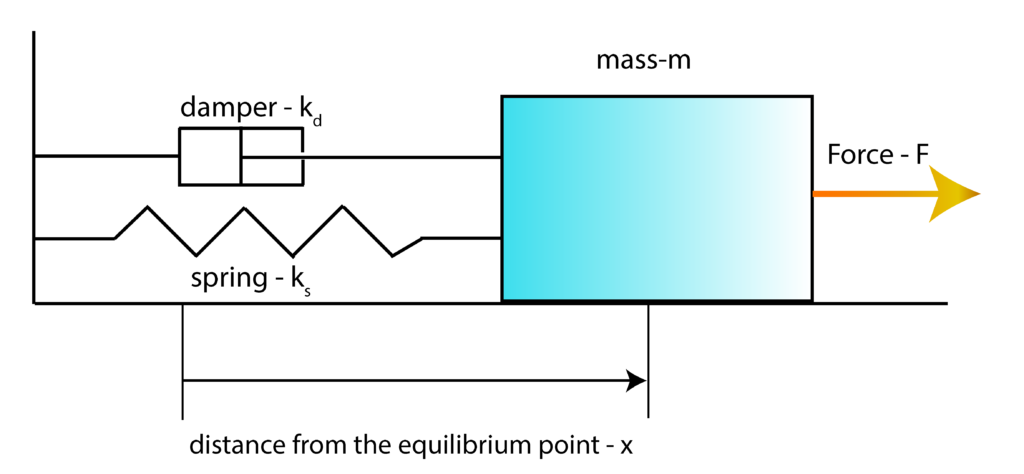
First, we introduce the state-space variables
\begin{align}
x_{1}=x \\
x_{2}=\dot{x}
\label{stateVariables}
\end{align}
where $\dot{x}=\frac{dx}{dt}$. Then, by using these state-space variables and by using the differential equation describing the system dynamics (see our previous post), we obtain the state-space model
\begin{align}
\underbrace{\begin{bmatrix}\dot{x}_{1} \\ \dot{x}_{2} \end{bmatrix}}_{\dot{\mathbf{x}}} &= \underbrace{\begin{bmatrix} 0 & 1\\ -\frac{k_{s}}{m} & -\frac{k_{d}}{m} \end{bmatrix}}_{A} \underbrace{\begin{bmatrix}x_{1} \\ x_{2} \end{bmatrix}}_{x}+\underbrace{\begin{bmatrix} 0 \\ \frac{1}{m}\end{bmatrix}}_{B}\underbrace{F}_{u} \\
\dot{\mathbf{x}}& =A\mathbf{x}+B\mathbf{u}
\label{SSmodelNew1}
\end{align}
Since in this post, we are considering state feedback, the output equation is not relevant. However, for completeness, we will write the output equation
\begin{align}
y=\underbrace{\begin{bmatrix} 1 & 0 \end{bmatrix}}_{C}\underbrace{\begin{bmatrix} x_{1} \\ x_{2} \end{bmatrix}}_{\mathbf{x}}+\underbrace{0}_{D}\cdot\underbrace{F}_{u}
\label{OutputEquation2222}
\end{align}
In this particular post and lecture, we assume that the full state information is available at every time instant. That is, we assume that both $x_{1}$ and $x_{2}$ are available. Everything presented in this lecture can be generalized for the case in which only position $x_{1}$ is observed.
The goal of the set point regulation is to steer the system to the desired state (desired set point) $\mathbf{x}_{D}$, starting from some non-zero initial state (that is in the general case different from $\mathbf{x}_{D}$) and under a possible action of external disturbances.
In this post, we will use the terms “desired state” and “desired set point” interchangeably. The first step is to determine the control input $\mathbf{u}_{d}$ that will produce the desired state $\mathbf{x}_{D}$ in the steady state. Since $\mathbf{x}_{D}$ is constant, by substituting $\mathbf{x}$ by $\mathbf{x}_{D}$, and $\mathbf{u}$ by $\mathbf{u}_{D}$ in (??), we obtain the following equation
\begin{align}
0= A\mathbf{x}_{D}+B\mathbf{u}_{D}
\label{equation1Derivation}
\end{align}
where $\dot{\mathbf{x}}_{D}=0$ since $\mathbf{x}_{D}$ is a constant steady-state. Assuming that the matrix $B$ has full column rank, from (??), we have that the desired control input $\mathbf{u}_{D}$, producing the desired steady-state $ \mathbf{x}_{D} $, is given by
\begin{align}
\mathbf{u}_{D} = – (B^{T} B)^{-1} B^{T} A\mathbf{x}_{D}
\label{desiredControlInput}
\end{align}
In principle, we can control the system by applying the constant control input $ \mathbf{u}_{D} $ and by waiting for the system to settle down in the desired steady-state $\mathbf{x}_{D}$. However, there are several issues with this type of control that can be exaggerated for undamped systems. Namely, the system might exhibit a large overshoot during its transient response, or oscillatory behavior. These phenomena can compromise system safety or performance. Furthermore, the system might be subjected to external disturbances that can seriously deteriorate the control accuracy and performance. These facts motivate the development of the set point feedback control algorithm. The idea is to improve the transient system response and disturbance rejection using a feedback control algorithm.
To develop the control algorithm, we introduce the error variables as follows
\begin{align}
\tilde{\mathbf{x}}=\mathbf{x}-\mathbf{x}_{D},\;\; => \;\; \mathbf{x} = \tilde{\mathbf{x}} + \mathbf{x}_{D} \\
\tilde{\mathbf{u}}=\mathbf{u}-\mathbf{u}_{D},\;\; => \;\; \mathbf{u} = \tilde{\mathbf{u}} + \mathbf{u}_{D}
\label{errorVariables}
\end{align}
By differentiating these expressions and by substituting (??) in (??), we obtain
\begin{align}
\dot{\mathbf{x}}= \dot{\tilde{\mathbf{x}}}+ \dot{\mathbf{x}}_{D}=A(\tilde{\mathbf{x}}+ \mathbf{x}_{D}) +B(\tilde{\mathbf{u}}+\mathbf{u}_{D})
\label{StateDerivation}
\end{align}
Here it should be kept in mind that since $\mathbf{x}_{D}$ is constant, we have $\dot{ \mathbf{x}}_{D}=0$. By substituting this in (??), we obtain
\begin{align}
\dot{\tilde{\mathbf{x}}} = A\tilde{\mathbf{x}}+B\tilde{\mathbf{u}}+A\mathbf{x}_{D}+B\mathbf{u}_{D}
\label{expressionDerivation}
\end{align}
On the other hand, by substituting (??) in (??), we obtain
\begin{align}
\dot{\tilde{\mathbf{x}}} = A\tilde{\mathbf{x}}+B\tilde{\mathbf{u}}
\label{substitutedValues}
\end{align}
Having this form of dynamics, we can straightforwardly apply the LQR algorithm that is derived under the assumption of zero desired state. The LQR algorithm optimizes the following cost function
\begin{align}
J(\tilde{\mathbf{u}})=\int_{t=0}^{t=\infty}\Big(\mathbf{\tilde{x}}^{T}Q \mathbf{\tilde{x}} + \mathbf{\tilde{u}}^{T}R \mathbf{\tilde{u}} +2 \mathbf{\tilde{x}}^{T}N \mathbf{\tilde{u}} \Big) \; dt
\label{costFunctionLQR}
\end{align}
where $Q$, $R$, and $N$ are the weighting matrices. The cost function is constrained by the system dynamics (??). The weighting matrices should be selected by the user and they need to satisfy a few assumptions (as well as the system matrices for the solution of the LQR problem to exist, however, in order not to blur the main ideas of this post with unnecessary mathematical perplexities, we will not discuss further these conditions). The matrix $Q$ penalizes the control error, and generally speaking, larger values of $Q$ will increase the speed of the system response. However, the trade-off is that more control energy will be spent to steer the system to the zero state. On the other hand, the matrix $R$ penalizes the control energy. Larger values of $R$ will generally minimize the control energy, however, at the expense of reducing the system’s response speed. In our simulations, we will assume that $N$ is a zero matrix. Furthermore, to simplify the control design, we will assume that the weighting matrices are diagonal. That is, we assume that
\begin{align}
Q=q\cdot I, \;\; R=r \cdot I
\end{align}
where $I$ is an identity matrix, and $q>0$ and $r>0$ are positive real numbers. The solution that optimizes the cost function (??) is the feedback control law of the following form
\begin{align}
\tilde{\mathbf{u}}=-K\tilde{\mathbf{x}}
\label{feedbackControlLaw}
\end{align}
where the matrix $K$ is defined by
\begin{align}
K=R^{-1}(B^{T}S+N^{T})
\label{matrixKcomputed}
\end{align}
where $S$ is the solution of the algebraic matrix Riccati equation:
\begin{align}
A^{T}S+SA-(SB+N)R^{-1}(B^{T}S+N^{T})+Q=0
\label{algebraicRiccatiEquation}
\end{align}
Fortunately, we do not need to write our own code for solving the Riccati equation. We will use the Python Control System Toolbox function control.lqr() to compute the control matrix $K$. By substituting (??) in (??), we obtain the closed-loop system
\begin{align}
\dot{\tilde{\mathbf{x}}}=(A-BK)\tilde{\mathbf{x}}
\label{closedLoopSystem}
\end{align}
The LQR control algorithm will make the matrix $A-BK$ asymptotically stable (all the eigenvalues of A-BK are in the left-half of the complex plane). This means that the set-point state error $\tilde{\mathbf{x}}$ will asymptotically approach zero. That is, in the steady-state, the system state $\mathbf{x}$ will become $\mathbf{x}_{D}$. From (??) , we have
\begin{align}
\dot{\mathbf{x}}=(A-BK)\mathbf{x}- (A-BK) \mathbf{x}_{D}
\label{ closedLoopSystem2}
\end{align}
The equation (??) can be used to simulate the closed loop system.
Taking into account the error variables (??), we can write the feedback control (??), as follows
\begin{align}
\mathbf{u}=\mathbf{u}_{D}-K(\mathbf{x}-\mathbf{x}_{D})
\label{feedbackControlAlgorithm}
\end{align}
Python Implementation
To install the Control Systems Library for Python, we need to open a terminal, and type:
pip install control
Next, open your favorite Python editor and start typing the code. First, we need to import the necessary libraries and define the plotting function. This is done by using the following Python script:
import matplotlib.pyplot as plt
import control as ct
import numpy as np

# this function is used for plotting of responses
# it generates a plot and saves the plot in a file

# xAxisVector - time vector
# yAxisVector - response vector
# titleString - title of the plot
# stringXaxis - x axis label
# stringYaxis - y axis label
# stringFileName - file name for saving the plot, usually png or pdf files

def plottingFunction(xAxisVector,
                     yAxisVector,
                     titleString,
                     stringXaxis,
                     stringYaxis,
                     stringFileName):

    plt.figure(figsize=(8,6))
    plt.plot(xAxisVector,yAxisVector, color='blue',linewidth=4)
    plt.title(titleString, fontsize=14)
    plt.xlabel(stringXaxis, fontsize=14)
    plt.ylabel(stringYaxis,fontsize=14)
    plt.tick_params(axis='both',which='major',labelsize=14)
    plt.grid(visible=True)
    plt.savefig(stringFileName,dpi=600)
    plt.show()
Here it is important to emphasize that the Python Control Systems Library is imported as
import control as ct
“ct” is the standard convention for importing the Control Systems Library. The plotting function “plottingFunction” will be used to plot the time response graphs and this function will save the result in the png file called: “stringFileName”. We define our state-space model as follows:
# parameters
m=10
ks=100
kd=5


# system matrices
A=np.array([[0, 1],[-ks/m, -kd/m]])
B=np.array([[0],[1/m]])
C=np.array([[1,0]])
D=np.array([[0]])

# define the state-space model
sysStateSpace=ct.ss(A,B,C,D)

#define the initial condition
x0=np.array([[0],[0]])

# print the system
print(sysStateSpace)
We define the system matrices and we use the function “ct.ss()” to define the state space model. We also define an initial condition x0 for simulation.
Next, we compute the step response of our system. This is done by using the following script:
# define the time vector for simulation
startTime=0
endTime=20
numberSamples=500
timeVector=np.linspace(startTime,endTime,numberSamples)

# define the control input vector for simulation
controlInputVector=np.ones(numberSamples)

# simulate the system
# 1 input argument - state-space model
# 2 input argument - time vector
# 3 input argument - defined control input
# 4 input argument - initial state for simulation
returnSimulation = ct.forced_response(sysStateSpace,
                                      timeVector,
                                      controlInputVector,
                                      x0)


# outputs of the forced_response is
# the TimeResponseData object consisting of
# time values of returned objects
returnSimulation.time
# computed outputs of the system
returnSimulation.outputs
# state sequence of the system
returnSimulation.states
# inputs used for simulation
returnSimulation.inputs

# plot the output
plottingFunction(returnSimulation.time,
                 returnSimulation.states[0,:],
                 titleString='Open-loop Response',
                 stringXaxis='time [s]' ,
                 stringYaxis='State 1 - Open Loop',
                 stringFileName='state1ResponseOL.png')


# plot the state 2
plottingFunction(returnSimulation.time,
                 returnSimulation.states[1,:],
                 titleString='Open-loop Response',
                 stringXaxis='time [s]' ,
                 stringYaxis='State 2 - Open Loop',
                 stringFileName='state2ResponseOL.png')
To compute the step response, we first define time (“timeVector”) and input vectors (“controlInputVector”). Then, we use the function “ct.forced_response()” to simulate the response of the system. The output of the function “ct.forced_response()” is the structure “returnSimulation”. The variables stored in this structure are:
- “returnSimulation.time”- time vector used for simulation
- “returnSimulation.outputs”- computed outputs
- “returnSimulation.states” – returned state sequence
- “returnSimulation.inputs” – returned inputs
We plot the state 1 ($x_{1}$) and state 2 ($x_{2}$). The results are shown below
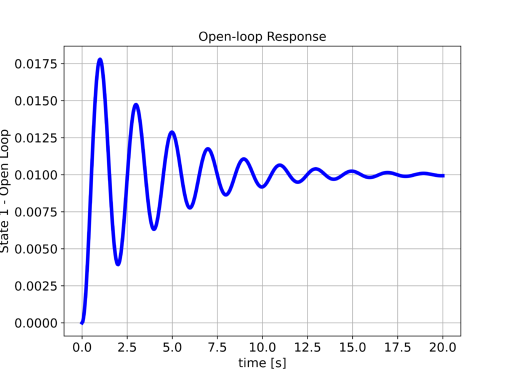
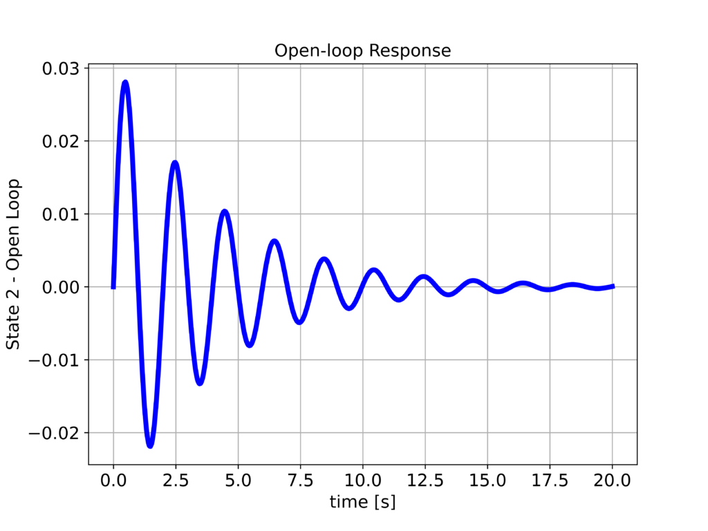
We can observe that the step response is not satisfactory:
- The system is not well-damped
- Also, there is a significant attenuation. We expect that the position $x_{1}$ will settle at 1. However, it settles at a much smaller value.
Next, we select the desired steady state and compute the steady-state desired input by using (??). The desired state is $x_{1D}=2$ and $x_{2D}=0$. The following Python script performs these tasks, and it computes the step response.
###############################################################################
# Determine the steady-state control input, and simulate
# the system
###############################################################################


# define the desired state
xd=np.array([[2],[0]])

M1=np.matmul(np.linalg.inv(np.matmul(B.T,B)),B.T)
M2=np.matmul(M1,A)

ud=-np.matmul(M2,xd)

timeVector=np.linspace(startTime,endTime,numberSamples)

# define the control input vector for simulation
controlInputVector=ud[0,0]*np.ones(numberSamples)

# simulate the system
# 1 input argument - state-space model
# 2 input argument - time vector
# 3 input argument - defined control input
# 4 input argument - initial state for simulation
returnSimulation = ct.forced_response(sysStateSpace,
                                      timeVector,
                                      controlInputVector,
                                      x0)


# plot the output
plottingFunction(returnSimulation.time,
                 returnSimulation.states[0,:],
                 titleString='Open-loop Response',
                 stringXaxis='time [s]' ,
                 stringYaxis='State 1 - Open Loop',
                 stringFileName='state1ResponseOLinput.png')


# plot the state 2
plottingFunction(returnSimulation.time,
                 returnSimulation.states[1,:],
                 titleString='Open-loop Response',
                 stringXaxis='time [s]' ,
                 stringYaxis='State 2 - Open Loop',
                 stringFileName='state2ResponseOLinput.png')
The following two graphs show the response when the constant $u_{D}$ is applied to the system.
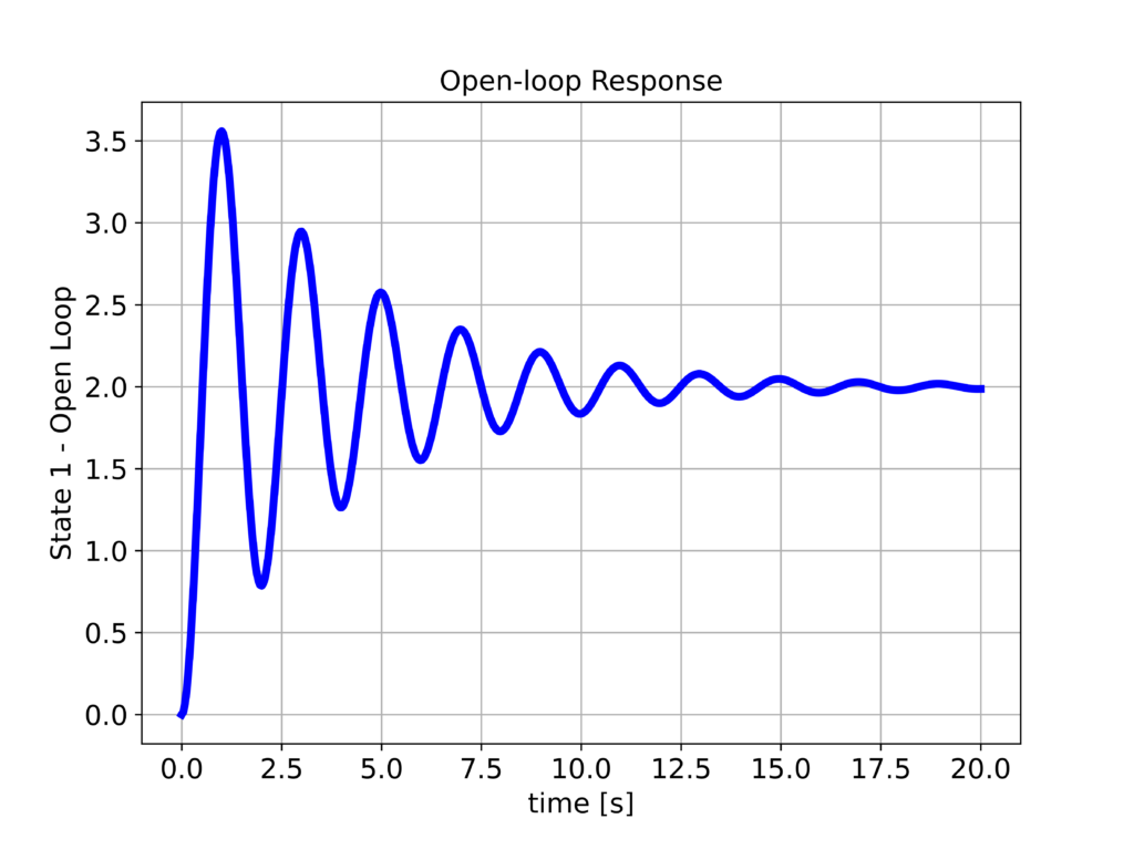

We have observed that the system position $x_{1}$ reaches the desired position equal to $2$. However, we can still observe the undamped response of the system. To improve the step response, we design the LQR controller by using the following Python script.
##############################################################
# design the LRQ controller
##############################################################


# state weighting matrix
Q=100*np.array([[10,0],[0,10]])

# input weighting matrix
R=1*np.array([[1]])

# K - gain matrix
# S - solution of the Riccati equation
# E - closed-loop eigenvalues

K, S, E = ct.lqr(sysStateSpace, Q, R)

Acl=A-np.matmul(B,K)
Bcl=-Acl
Dcl=np.array([[0,0]])

# define the state-space model
sysStateSpaceCl=ct.ss(Acl,Bcl,C,Dcl)


# define the time vector for simulation
timeVector=np.linspace(startTime,endTime,numberSamples)

# define the input for closed-loop simulation
inputCL=np.zeros(shape=(2,numberSamples))
inputCL[0,:]=xd[0,0]*np.ones(numberSamples)
inputCL[1,:]=xd[1,0]*np.ones(numberSamples)


returnSimulationCL = ct.forced_response(sysStateSpaceCl,
                                      timeVector,
                                      inputCL,
                                      x0)

# plot the output
plottingFunction(returnSimulationCL.time,
                 returnSimulationCL.states[0,:],
                 titleString='Closed-loop Response',
                 stringXaxis='time [s]' ,
                 stringYaxis='State 1 - Closed Loop',
                 stringFileName='state1ResponseCL.png')


# plot the state 2
plottingFunction(returnSimulationCL.time,
                 returnSimulationCL.states[1,:],
                 titleString='Closed-loop Response',
                 stringXaxis='time [s]' ,
                 stringYaxis='State 2 - Closed Loop',
                 stringFileName='state2ResponseCL.png')
To design the LQR controller, we use the function :
K, S, E = ct.lqr(sysStateSpace, Q, R)
The first input argument of this function is our state space model. However, the state-space model is not the original state-space model. Instead, we define the closed-closed loop system defined by (\eqref{closedLoopSystem2}). The input to this state-space model is the desired steady-state $\mathbf{x}_{D}$. Consequently, we redefined the system matrices such that they match the state-space matrices of this model. The second and third arguments are the weighting matrices Q and R which are chosen as diagonal matrices. The control design function returns the following variables:
- “K” feedback control matrix
- “S” solution of the Riccati equation (??)
- “E” vector of closed loop poles. That is, the vector of eigenvalues of $A-KC$.
The closed-loop system response computed by using the above Python script is shown below.
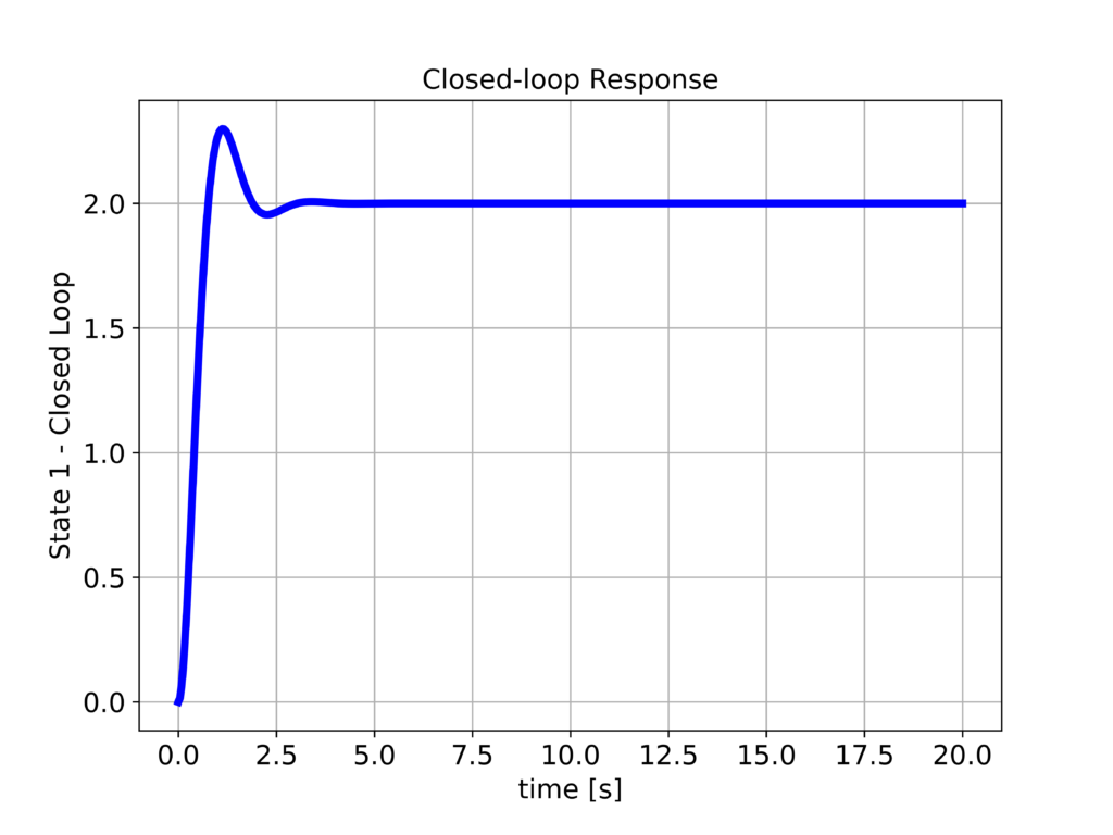
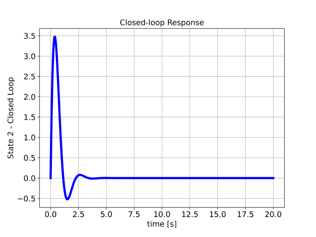
From the first figure above, we can observe that the response is relatively well-damped, and we can see a significant improvement in the system response compared to the open-loop responses.