by
by
In this control engineering, control theory, and process control tutorial, we explain how to develop a dynamical model of a tank (reservoir) filled with a liquid and how to simulate such a model in Python. This is a classical problem for understanding the dynamics of fluid and process systems. The YouTube video accompanying this tutorial is given below.
Problem Formulation
The figure given below introduces the problem.
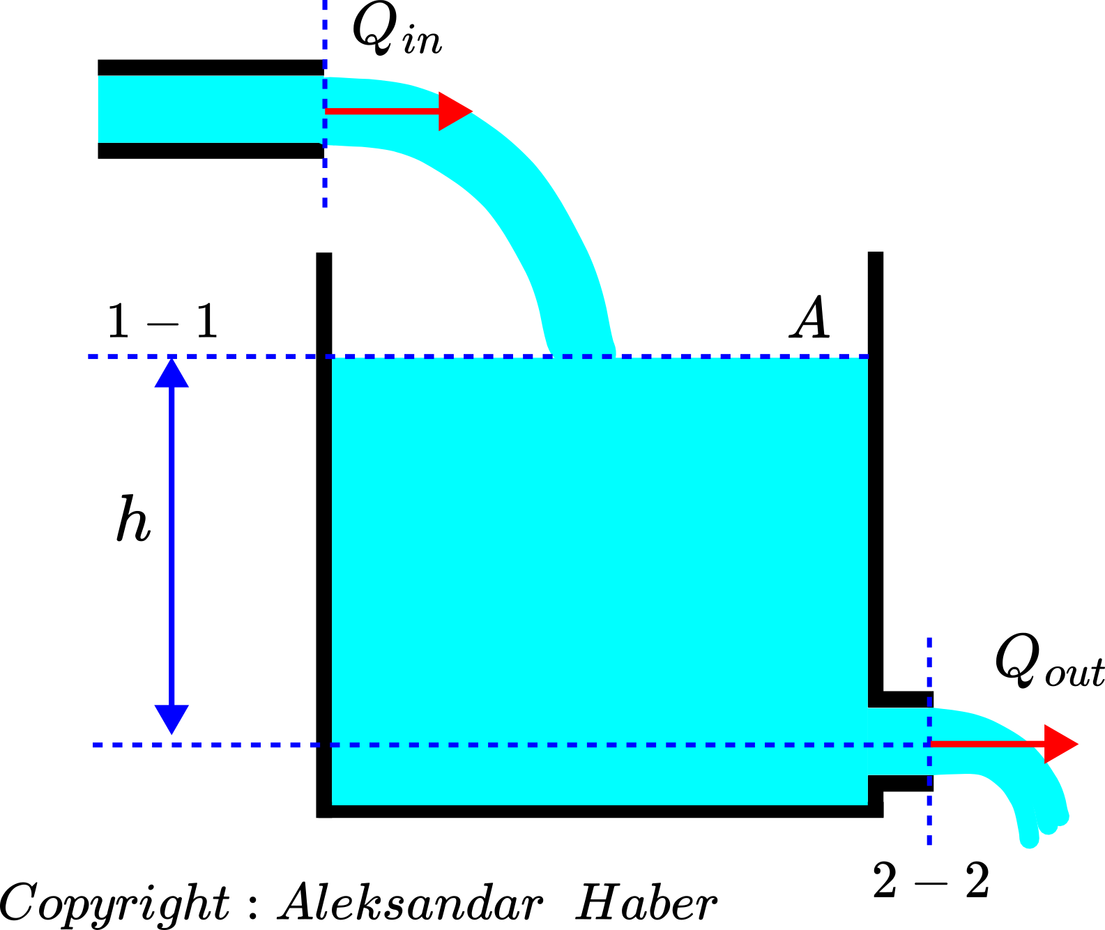
We consider a tank with a cross-section area of  filled with an incompressible fluid. The fluid level at the time instant
  is
is  . The input (volumetric) flow rate to the tank is denoted by
  . The output (volumetric) flow rate of the tank is denoted by
  . We assume that the output flow is passive (not actively controlled). We assume that the cross-section of the hole is much smaller than the cross-section of the tank. We assume that we can control the input flow rate . Our goal is
- Derive a differential equation describing the change of the fluid level as the function of time and as the function of .
- For a given initial fluid level
 and for a given time series of , numerically solve and simulate the solution of the derived differential equation in Python.
Modeling and Simulation of a Tank Model in Python
Consider the figure given below.
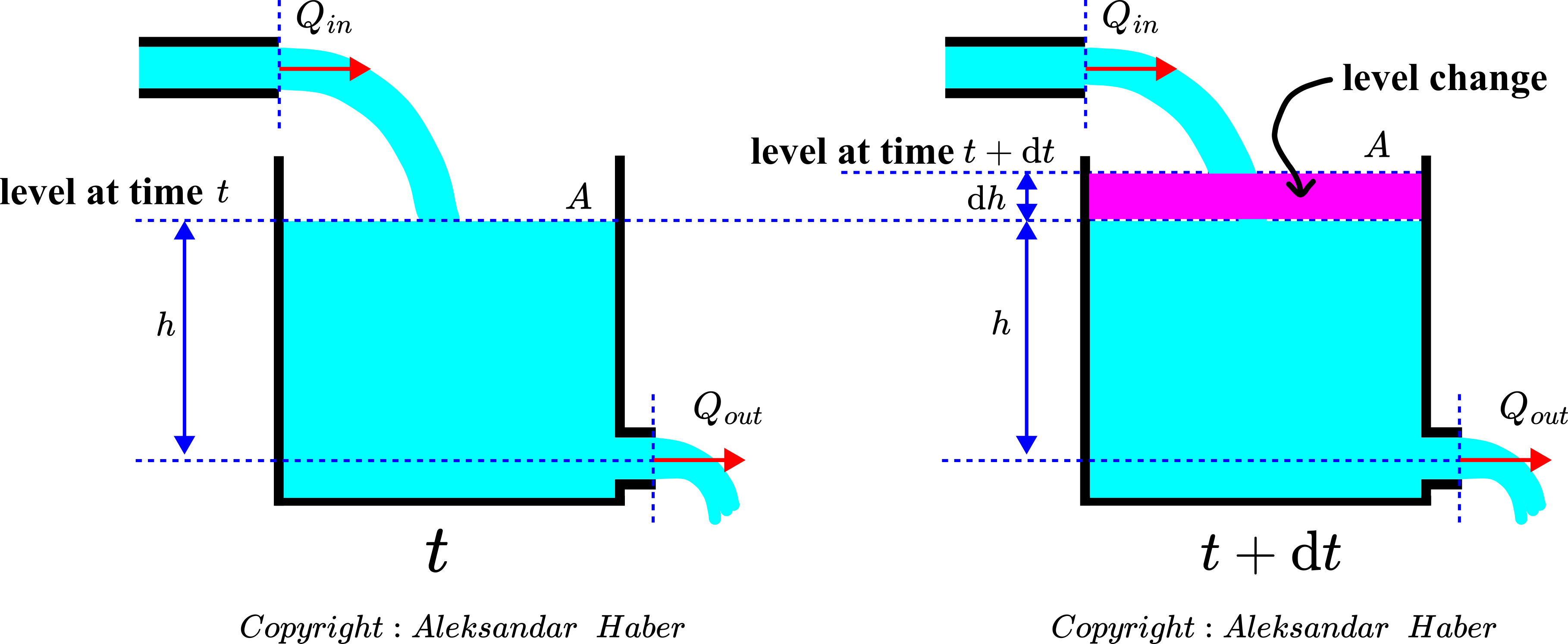 . Right – fluid level at the time instant
  .
.On the left part of the figure, we show the fluid level at the time instant . After an infinitesimally small amount of time  , due to the input flow the fluid level changed to
  , where
  is the change of the fluid level. The volume change is
  .
.
The rate of change of the fluid volume during this time instant is
(1) 
On the other hand, the term
(2) 
is the velocity of the fluid in the tank.
On the other hand, in the general case, the flow is the product of the fluid velocity and the area through which the fluid flows. That is
(3) 
where  is the area and
  is the velocity of the fluid. Taking all these things into account, we conclude that the product in (1) is actually a total flow of the fluid in the tank. This flow is actually a difference between the flow coming in and the flow getting out of the tank. That is,
(4) 
On the other hand, since the output flow is passive, we can use a formula in our previous tutorial for the output flow. This formula is
(5) 
where  is the discharge coefficient and
  is the gravitational acceleration constant. We write the last equation as follows:
(6) 
where the constant  is defined by
(7) 
By substituting (6) in (4), we obtain the model of the tank system:
(8) 
The last equation can be written in the following form
(9) 
This is the final form we use for the simulation of the system in Python. The Python code for simulating the system is explained in the video above and after paying a small fee, the code can be accessed by using this link.
We assume the following simulation conditions. The initial height  (all the units are SI units). The area is
  . The constant
The input flow is given in the figure below.
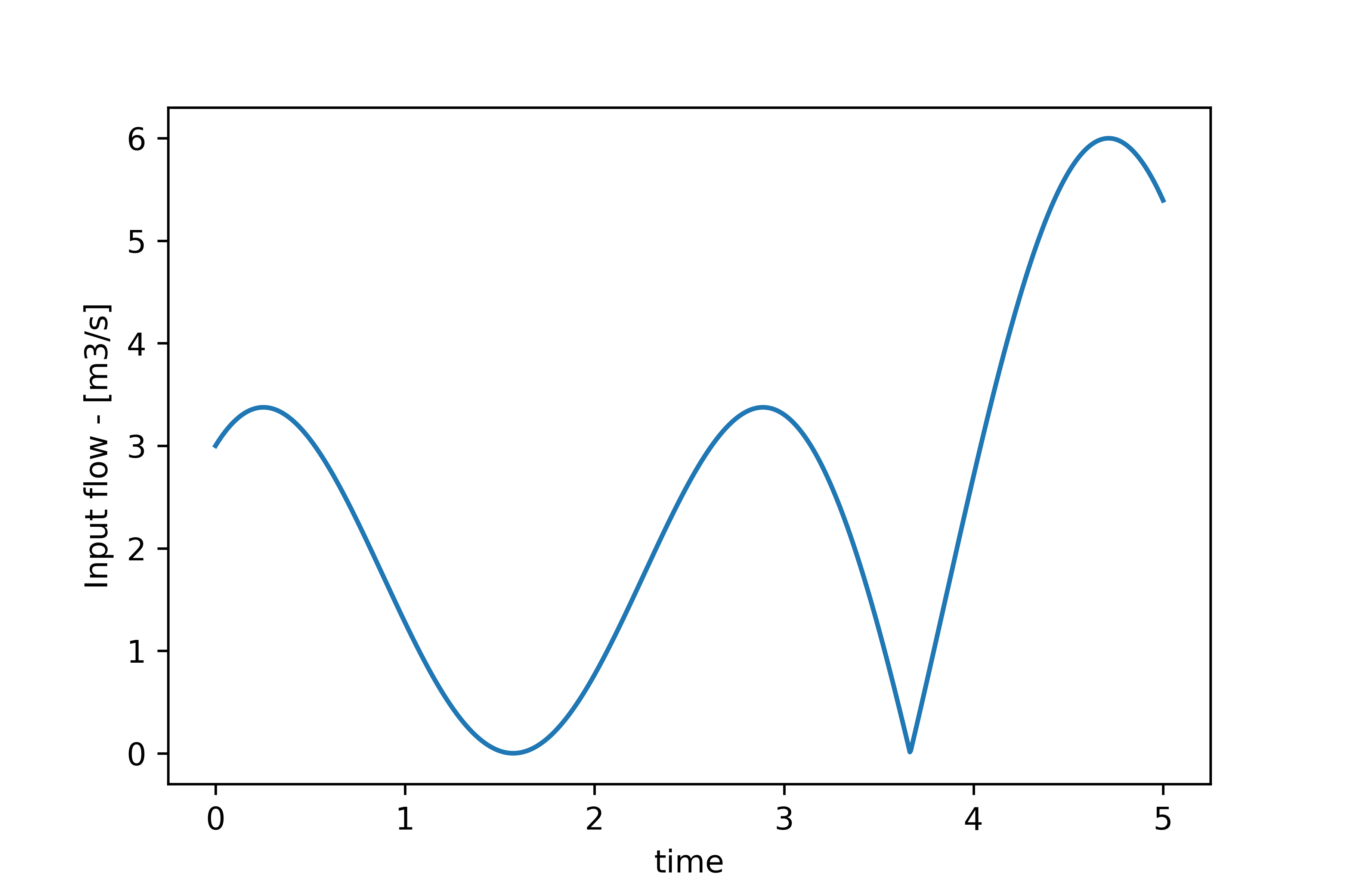 used for simulation.
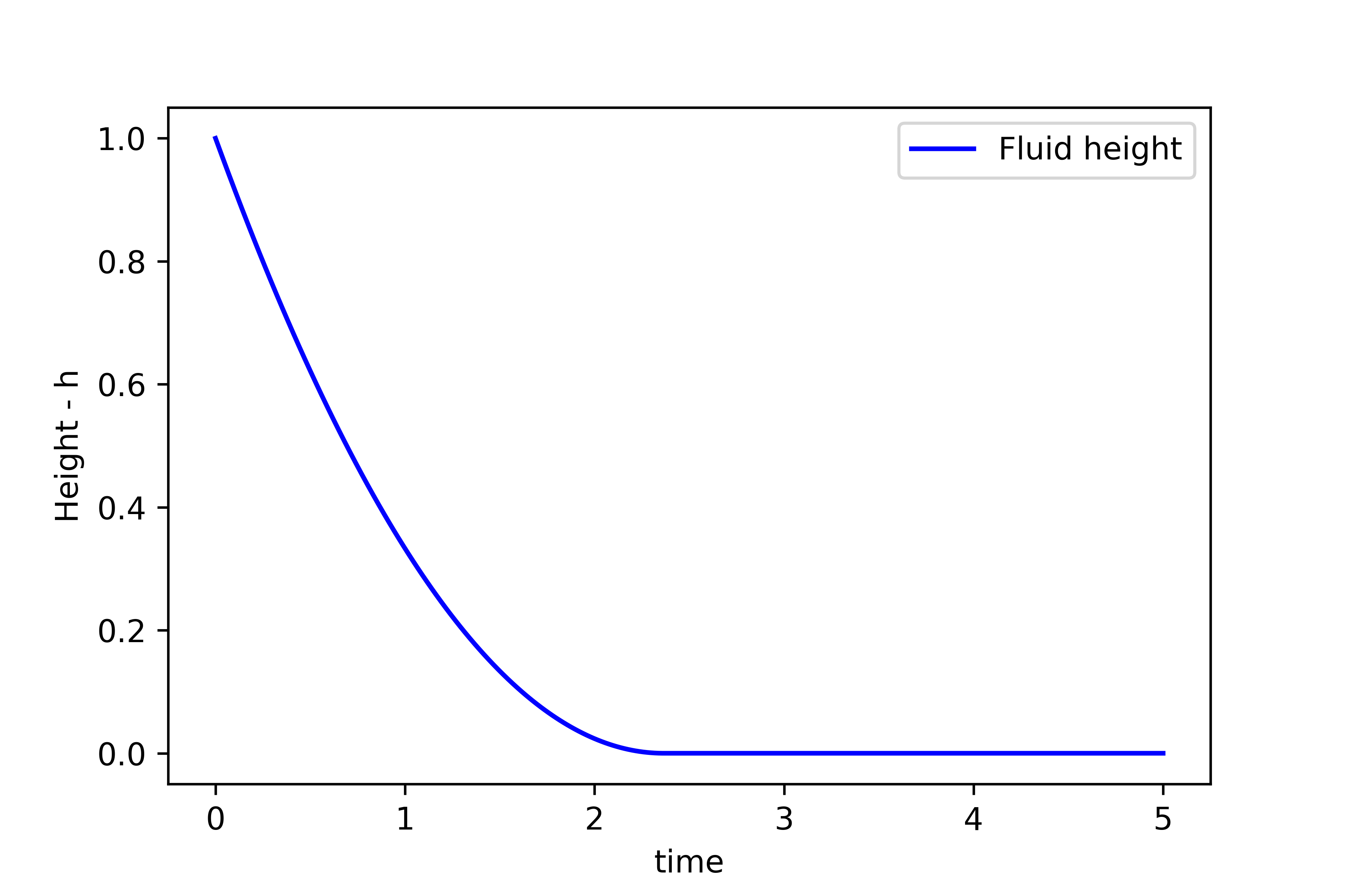
The simulated height is given in the figure below.
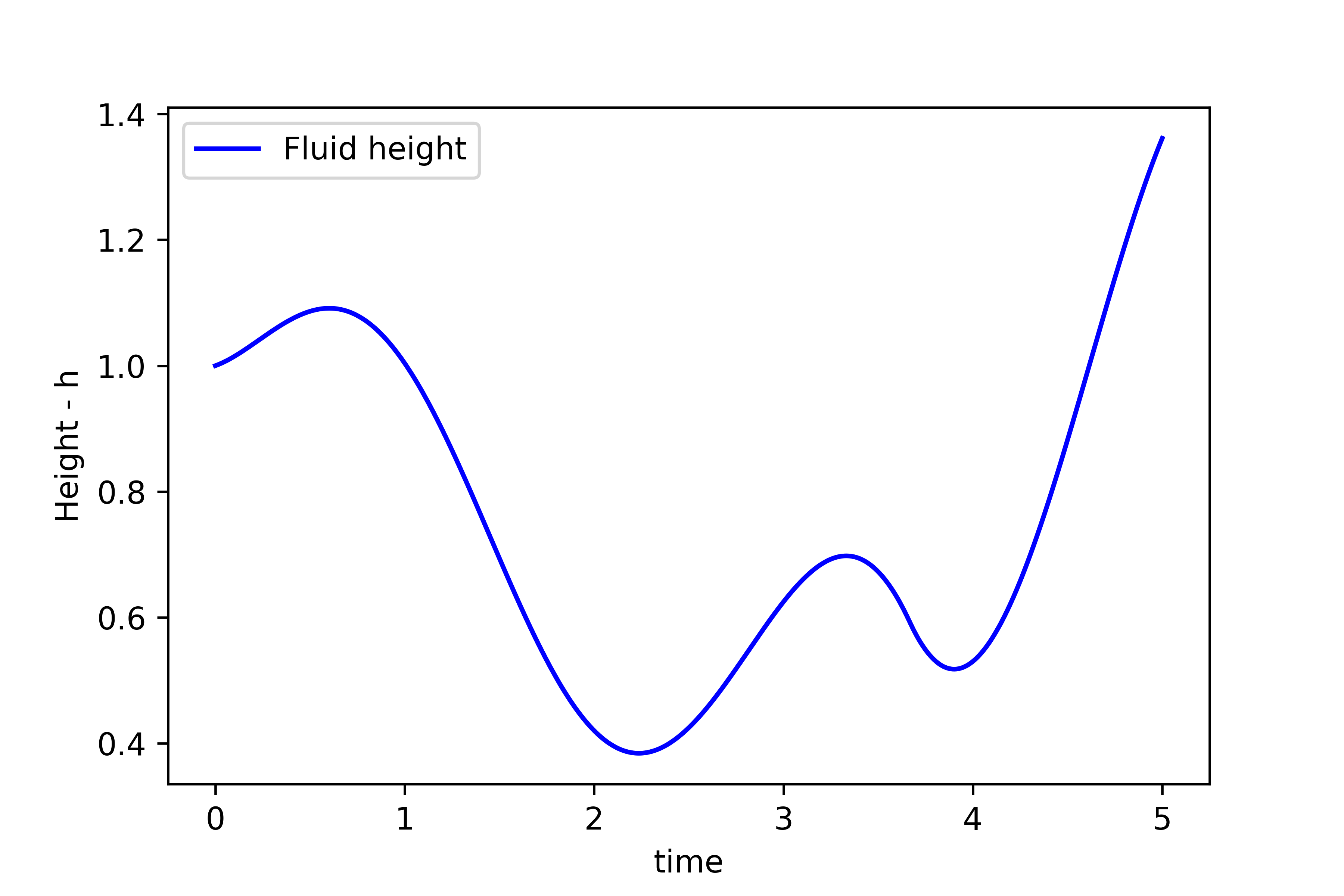
Next, we simulate the response of the system to the initial state. The results are shown below.