Easy Introduction to Observability and Open-loop Observers with MATLAB Implementation – Fusion of Engineering, Control, Coding, Machine Learning, and Science

In this tutorial, we provide a brief introduction to open-loop observers. In this tutorial, you will learn

The concept of observability.
How to estimate an initial state of a linear dynamical system by using an open-loop observer.
How to properly understand the concept of numerical observability.

The motivation for creating this tutorial comes from the fact that students often have difficulties understanding the concept of observability and they often do not understand the need for observers. This comes from the fact that the concept of observability is often first taught by assuming continuous-time systems. The mathematics needed to describe continuous-time systems is more complex than the mathematics necessary to describe discrete-time systems. It involves integrals applied to vector and matrix expressions that often involve matrix exponentials. These concepts might be difficult to understand for an average engineering student.

Instead of introducing the concept of observability by assuming a continuous-time system, we will present this concept by assuming a discrete-time system. In this way, we significantly simplify the mathematics necessary to understand the basic concepts.

So let us immediately explain the need for observability analysis by considering the example shown in the figure below.

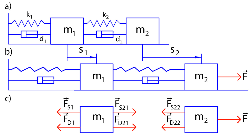
Figure 1: Double mass-spring system used to illustrate the concept of observability.

The above figure illustrates a prototypical model of two masses connected with springs and dampers. There is a force $F$ moving the second mass. The equations governing the behavior of this system are very similar to the equations of motion of a number of mechanical and electrical systems, such as electrical and electronics circuits, mechanical systems whose motion is described by Newton’s equations, robotic arms, etc.

In our previous post, whose link is given here, we have derived a state-space model of this system. The states are:

(1) $\begin{align*}x_{1}=\text{position of the first mass} = s_{1} \\x_{2}=\text{velocity of the first mass}=\dot{s}_{1} \\x_{3}=\text{position of the second mass}=s_{2} \\x_{4}=\text{velocity of the second mass}=\dot{s}_{2} \\ \end{align*}$

In order to develop a feedback control it is often necessary to obtain information about all the states: $x_{1},x_{2},x_{3}$ and $x_{4}$ . However, in practice, we can only observe a single state variable, such as, for example, position $x_{1}$ or $x_{3}$ . The observability analysis tries to provide the answers to these types of questions

Is it possible to reconstruct the full state vector (all state variables $x_{1},x_{2},x_{3}$ and $x_{4}$ ) by only measuring the position of the first mass over time? That is, is it possible to reconstruct time series $x_{2},x_{3}$ and $x_{4}$ by only observing the time series of $x_{1}$ ?
If it is not possible to reconstruct all other state variables by only measuring $x_{1}$ , then how many state variables do we need to observe to reconstruct the full state vector?

Consider the following linear discrete-time system

(2) $\begin{align*}\mathbf{x}_{k+1}=A\mathbf{x}_{k} \\\mathbf{y}_{k}=C\mathbf{x}_{k}\end{align*}$

where $\mathbf{x}_{k}\in \mathbb{R}^{n}$ is the system state at the discrete-time sample $k$ , $\mathbf{y}_{k}\in \mathbb{R}^{r}$ is the output of the system at the discrete-time sample $k$ , and $A$ and $C$ are system matrices. The system output $\mathbf{y}_{k}$ is usually observed by a sensor. However, the state of the system $\mathbf{x}_{k}$ is usually not directly observable.

Note that we have assumed that the inputs are not affecting our system dynamics. This is done for presentation clarity since the inputs do not affect the system observability. We can also easily modify our approach to include the system’s inputs.

Let us consider the following problem. Our task is to estimate the system’s initial state $\mathbf{x}_{0}$ , (the system state $\mathbf{x}_{k}$ at the discrete-time sample $k=0$ ), from the sequence of the observed outputs $\mathbf{y}_{0},\mathbf{y}_{1},\mathbf{y}_{2},\ldots, \mathbf{y}_{M-1}$ , where $M$ is the total number of outputs (observations). This problem is in fact the observability problem for the discrete time system (2)

So how to mathematically formulate and solve this problem?

By propagating the state equation of the system (2) in discrete-time, we have

(3) $\begin{align*}\mathbf{x}_{k+1}&=A\mathbf{x}_{k} \\\mathbf{x}_{k+2}&=A^{2}\mathbf{x}_{k}\\\vdots \\\mathbf{x}_{k+M-1}&=A^{M-1}\mathbf{x}_{k}\\\end{align*}$

Combining these equations with the output equation, we obtain

(4) $\begin{align*}\mathbf{y}_{k}& =C\mathbf{x}_{k} \\\mathbf{y}_{k+1} & =CA\mathbf{x}_{k} \\\mathbf{y}_{k+2}& =CA^{2}\mathbf{x}_{k}\\\vdots \\\mathbf{y}_{k+M-1}& =CA^{M-1}\mathbf{x}_{k}\\\end{align*}$

These equations can be written in the vector-matrix form

(5) $\begin{align*}\begin{bmatrix}\mathbf{y}_{k} \\ \mathbf{y}_{k+1} \\ \vdots \\ \mathbf{y}_{k+M-1} \end{bmatrix}=\begin{bmatrix}C \\ CA \\ CA^{2} \\ \vdots \\ CA^{M-1} \end{bmatrix}\mathbf{x}_{0}\end{align*}$

The last equation can be written compactly

(6) $\begin{align*}\mathbf{y}_{k:k+M-1}=O_{M}\mathbf{x}_{k}\end{align*}$

where

(7) $\begin{align*}\mathbf{y}_{k:k+M-1}=\begin{bmatrix}\mathbf{y}_{k} \\ \mathbf{y}_{k+1} \\ \vdots \\ \mathbf{y}_{k+M-1} \end{bmatrix},\;\; O_{M}=\begin{bmatrix}C \\ CA \\ CA^{2} \\ \vdots \\ CA^{M-1} \end{bmatrix}\end{align*}$

When $M=n$ , where $n$ is the state order of the system, the matrix $O_{n}$ (matrix $O_{M}$ for M=n) is called the observability matrix.

The notation $\mathbf{y}_{k:k+M-1}$ denotes the lifted vector. Lifted vectors are formed by “lifting” underlying vectors over time. This means that the vector $\mathbf{y}_{k:k+M-1}$ is formed by stacking vectors $\mathbf{y}_{k}$ , $\mathbf{y}_{k+1}$ , $\ldots$ , $\mathbf{y}_{k+M-1}$ on top of each other. The subscript notation $k:k+M-1$ , means that the starting time instant for lifting is $k$ and the ending time instant is $k+M-1$ . By setting $k=0$ in (6), we obtain

(8) $\begin{align*}\mathbf{y}_{0:M-1}=O_{M}\mathbf{x}_{0} \end{align*}$

The last equation is important since it shows us that the observability problem is to determine the initial state $\mathbf{x}_{0}$ from the observation vector $\mathbf{y}_{0:M-1}$ . Since the last equation represents a system of linear equations, the observability problem is equivalent to the problem of solving the system of linear equations, where the unknown variables are entries of the vector $\mathbf{x}_{0}$ . In order to ensure that this system has a unique solution, or equivalently in order to ensure that the system is observable, in the most general case, it is necessary and sufficient that:

The number of observation samples $M$ is larger than or equal to $n$ , where $n$ is the system state order.
$\text{rank}\Big(O_{M}\Big)=n$ . This means that the observability matrix $O_{M}$ has full rank.

Here, a few important things should be kept in mind. Condition (1) is stated for the most general case. However, it might happen that the output dimension $r$ (the dimension of the vector $\mathbf{y}_{k}$ ) is such that we can ensure that the matrix $O_{M}$ has full rank even if $M<n$ . For example, consider this system

(9) $\begin{align*}\mathbf{x}_{k+1}=A\mathbf{x}_{k} \\ \mathbf{y}_{k}=I\cdot \mathbf{x}_{k}\end{align*}$

where $I\in \mathbb{R}^{n \times n}$ is an identity matrix. In the case of this system, $M=1$ , will ensure the system observability since the matrix $C$ is equal to the identity matrix, and identity matrices are invertible. In practice, it is not necessary to take the number of samples $M$ to be larger than $n$ . This is because the entries $CA^{M}$ for $M >n$ can be expressed as linear combinations of CA^{P}, where $P=0,1,2,\ldots, n$ . This follows from the Cayley-Hamilton theorem. However, in the presence of the measurement noise in the equation (2), it might be beneficial to take more samples $M$ (and $M$ should be larger than $n$ ), since, in this way, it is possible to decrease the sensitivity of estimating the initial state from the observed outputs.

Let us assume that the conditions (1) and (2) are satisfied. We can multiply the equation (8) from left by $O_{M}^{T}$ , and as the result, we obtain

(10) $\begin{align*}O_{M}^{T}\mathbf{y}_{0:M-1}=O_{M}^{T}O_{M}\mathbf{x}_{0} \end{align*}$

Then, since the matrix $O_{M}$ has a full column rank, the matrix $O_{M}^{T}O_{M}$ is invertible, and from (10), we obtain

(11) $\begin{align*}\mathbf{x}_{0}=\Big( O_{M}^{T}O_{M} \Big)^{-1}O_{M}^{T}\mathbf{y}_{0:M-1}\end{align*}$

The equation (11) is the solution to the observability problem. We have obtained an initial state estimate as a function of the observations: $\mathbf{y}_{0},\mathbf{y}_{1},\ldots, \mathbf{y}_{M-1}$ .

Now that we have informally introduced the concept of observability, we can give a formal definition:

Observability Definition: The system (2) is observable, if any initial state $\mathbf{x}_{k}$ is uniquely determined by the observed outputs $\mathbf{y}_{k},\mathbf{y}_{k+1},\mathbf{y}_{k+2},\ldots, \mathbf{y}_{k+M}$ , for some finite positive integer $M$ .

We can also state the observability rank condition:

Observability rank condition: The system (2) is observable if and only if $\text{rank}\Big(O_{n}\Big)=n$ .

From everything being said, it follows that we can check the observability condition by investigating the rank of the matrix $O_{n}$ .

However, this criterion has the following issue. Namely, formally speaking, the matrix might have a full rank, however, it might be close to the singular matrix. That is, its condition number might be very large or its smallest singular value might be close to zero. This implies that in order to investigate the observability of the system it is usually more appropriate to compute the condition number or the smallest singular value.

Let us numerically illustrate all these concepts by using the example from the beginning of this post. In our previous post, explaining the subspace identification method, we have introduced this example This example is briefly summarized below. For completeness, we repeat the figure illustrating this example.

The state-space model is given below

(12) $\begin{align*}\underbrace{\begin{bmatrix}\dot{x}_{1} \\ \dot{x}_{2} \\ \dot{x}_{3} \\ \dot{x}_{4}\end{bmatrix}}_{\dot{\mathbf{x}}}= \underbrace{\begin{bmatrix}0 & 1 & 0 & 0 \\ -\frac{k_{1}+k_{2}}{m_{1}} & -\frac{d_{1}+d_{2}}{m_{1}} & \frac{k_{2}}{m_{1}} & \frac{d_{2}}{m_{1}} \\0 & 0 & 0 & 1 \\ \frac{k_{2}}{m_{2}} & \frac{d_{2}}{m_{2}} & -\frac{k_{2}}{m_{2}} & -\frac{d_{2}}{m_{2}} \end{bmatrix}}_{A_{c}} \underbrace{\begin{bmatrix}x_{1} \\ x_{2} \\ x_{3} \\ x_{4}\end{bmatrix}}_{\mathbf{x}}+\underbrace{\begin{bmatrix} 0 \\ 0 \\ 0 \\ \frac{1}{m_{2}} \end{bmatrix}}_{B_{c}}\underbrace{F}_{\mathbf{u}} \end{align*}$

We assume that only the position of the first object can be directly observed. This can be achieved using for example, infrared distance sensors. Under this assumption, the output equation has the following form

(13) $\begin{align*}\mathbf{y}=\underbrace{\begin{bmatrix}1 & 0 & 0 & 0\end{bmatrix}}_{C}\mathbf{x}\end{align*}$

The next step is to transform the state-space model (12)-(13) in the discrete-time domain. Due to its simplicity and good stability properties we use the Backward Euler method to perform the discretization. This method approximates the state derivative as follows

(14) $\begin{align*}\frac{\mathbf{x}_{k}-\mathbf{x}_{k-1}}{h}=A_{c}\mathbf{x}_{k}+B_{c}\mathbf{u}_{k-1}\end{align*}$

where $h$ is the discretization time step. For simplicity, we assumed that the discrete-time index of the input is $k-1$ . We can also assume that the discrete-time index of input is $k$ . However, then, when simulating the system dynamics we will start from $k=1$ . From the last equation, we have

(15) $\begin{align*}\mathbf{x}_{k}=A\mathbf{x}_{k-1}+B \mathbf{u}_{k-1} \end{align*}$

where $A=(I-hA_{c})^{-1}$ and $B=hAB_{c}$ . On the other hand, the output equation remains unchanged

(16) $\begin{align*}\mathbf{y}_{k}=C\mathbf{x}_{k}\end{align*}$

We neglect the input and without the loss of generality, we shift the time index from $k$ to $k+1$ , and consequently, we obtain the final state-space model

(17) $\begin{align*}\mathbf{x}_{k+1}=A\mathbf{x}_{k} \\\mathbf{y}_{k}=C\mathbf{x}_{k}\end{align*}$

Next, we introduce the MATLAB code. First, we define the model parameters and other variables

clear,pack,clc
% model parameters
k1=10, k2=20, d1=0.5, d2=0.3, m1=10, m2=20
% discretization constant
h=0.1

% simulate the system 
simulationTime=500

% number of time steps for estimating the initial state
M=5

%% system matrices
Ac=[0 1 0 0;
    -(k1+k2)/m1 -(d1+d2)/m1 k2/m1 d2/m1;
    0 0 0 1;
    k2/m2 d2/m2 -k2/m2 -d2/m2]
C=[1 0 0 0]
[s1,s2]=size(C)
% discrete-time system
A=inv(eye(4)-h*Ac)

% select the initial state to be estimated
x0=[0.5;0.1;0; -0.4];

First, we define the model parameters such as damping, stifness and masses. We use a discretization constant of $h=0.1$ , and total simulation time of 500. Then, we define the system matrices $A$ and $C$ , and we define the discretized matrix $A$ . We define the initial state. This state is used to simulate the system response and we will estimate this initial state. We select $M=5$ time samples to form the lifted vectors and the observability matrix.

Next, we simulate the system response. The following code lines simulate the system response and form the obeservability matrix

%% simulate the system
stateVector=zeros(4,simulationTime+1); 
outputVector=zeros(s1,simulationTime+1); 

stateVector(:,1)=x0;
outputVector(:,1)=C*x0;

for i=1:simulationTime
    stateVector(:,i+1)=A*stateVector(:,i);
    outputVector(:,i+1)=C*stateVector(:,i+1);
end

% form the M-steps observability matrix

for i=1:M
    Obs{i,1}=C*A^(i-1); % M-steps observability matrix
    Y{i,1}=outputVector(:,i); % Lifted output vector
end

Obs=cell2mat(Obs);
Y=cell2mat(Y);

% plot the response
simulationTimeVector=0:h:h*simulationTime;
figure(1)
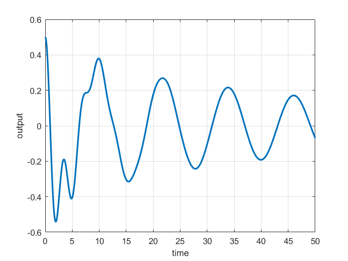
plot(simulationTimeVector,outputVector,LineWidth=2)
xlabel('time')
ylabel('output')
grid

The system response is shown in the figure below.

Figure 3: Simulated output of the system starting from the initial state.

Next, we estimate the initial state by using the equation (11). Then we compare the estimate with the initial state by computing the relative estimation error. Then, we compute the singular values of the observability matrix and compute the condition number.

% estimate the initial state
x0Est=inv(Obs'*Obs)*Obs'*Y

% compute the relative error
norm(x0Est-x0,2)/norm(x0,2)

% compute the singular value decomposition
[U,S,V] = svd(Obs);

% singular values
diag(S)

% condition number
cond(Obs)

You can modify this code by changing the structure of the C matrix. For example, you can investigate the effect of observing some other variable (for example, what happens when $C=\begin{bmatrix} 0 & 1 & 0 & 0 \end{bmatrix}$ ). This is explained in the accompanying YouTube video. Also, you can modify the number of observability steps and modify the system parameters.

2 thoughts on “Easy Introduction to Observability and Open-loop Observers with MATLAB Implementation”

Cakan says:

June 25, 2022 at 9:29 am

Is it possible to apply this observer in simulink?
admin says:

June 25, 2022 at 11:53 pm

Probably it is. However, I do not have enough time to investigate how to do this.

Comments are closed.

admin

You might also like

5. Accurately Compute Exponential Moving Averages in Pandas and Python

Installation and Getting Started with OpenAI Gym and Frozen Lake Environment – Reinforcement Learning Tutorial

Python Control Systems Library Tutorial 2: Define State-Space Models, Generate Step Response, Discretize, and Perform Basics Operations

2 thoughts on “Easy Introduction to Observability and Open-loop Observers with MATLAB Implementation”