Python Control Systems Library Tutorial 2: Define State-Space Models, Generate Step Response, Discretize, and Perform Basics Operations

In this control engineering and control theory tutorial, we provide an introduction to Python Control Systems Library. We explain how to

1. Define state-space models
2. Compute step responses
3. Compute step-response characteristics, such as rise time, settling time, overshoot, undershoot, etc.
4. Convert state-space models to transfer function models and vice-versa
5. Discretize the state-space model

The YouTube tutorial accompanying this webpage is given below.

Import libraries and Define the Plotting Function

First, we import the necessary libraries and define the plotting function that is used for plotting the step responses of the system.

import matplotlib.pyplot as plt
import control as ct
import numpy as np

# this function is used for plotting of responses 
# it generates a plot and saves the plot in a file 

# xAxisVector - time vector
# yAxisVector - response vector
# titleString - title of the plot
# stringXaxis - x axis label 
# stringYaxis - y axis label
# stringFileName - file name for saving the plot, usually png or pdf files

def plottingFunction(xAxisVector,yAxisVector,titleString,stringXaxis,stringYaxis,stringFileName):
    plt.figure(figsize=(8,6))
    plt.plot(xAxisVector,yAxisVector, color='blue',linewidth=4)
    plt.title(titleString, fontsize=14)
    plt.xlabel(stringXaxis, fontsize=14)
    plt.ylabel(stringYaxis,fontsize=14)
    plt.tick_params(axis='both',which='major',labelsize=14)
    plt.grid(visible=True)
    plt.savefig(stringFileName,dpi=600)
    plt.show()

Here it is important to emphasize that it is recommended by the creators of the Python Control Systems library to import the “control” library as “ct”. The function “plottingFunction” is used for plotting the step responses of the system. Note that this function will also save the graph to the file specified by the user.

Define State-Space Models and Convert State-Space Models to Transfer Functions and Vice-Versa

We define the state-space model by using the function ss()

A=np.array([[0, 1],[-4, -2]])
B=np.array([[0],[1]])
C=np.array([[1,0]])
D=np.array([[0]])

sysStateSpace=ct.ss(A,B,C,D)

print(sysStateSpace)

First, we define the state-space matrices as NumPy arrays, and we pass these matrices to the function ss().

We can convert state-space models to transer-functions and back, as follows:

# convert state-space to transfer function
transferFunction1=ct.ss2tf(sysStateSpace)
print(transferFunction1)

# convert transfer function to state-space 
sysStateSpace2=ct.tf2ss(transferFunction1)
print(sysStateSpace2)

The function ss2tf() is used for the conversion of the state-space model to the transfer function model. On the other hand, we can convert transfer functions to state-space models by using the function tf2ss(). Here, one important details should be observed. If we print the original state-space model “sysStateSpace”, we obtain

: sys[43]
Inputs (1): [‘u[0]’]
Outputs (1): [‘y[0]’]
States (2): [‘x[0]’, ‘x[1]’]

A = [[ 0. 1.]
[-4. -2.]]
B = [[0.]
[1.]]
C = [[1. 0.]]
D = [[0.]]

On the other hand, if we print the transformed state-space model “sysStateSpace2”, we obtain

A = [[-2. -4.]
[ 1. 0.]]

B = [[1.]
[0.]]

C = [[0. 1.]]

D = [[0.]]

The state-space matrices A,B, and C are different. However, these two systems are equivalent and they have identical dynamical properties (the identical step response and eigenvalues). In fact, there is a similarity transformation (state-space transformation) that can transfer one state-space model to another.

Response and Basic Computations

We can compute the step response of the system as follows

timeVector=np.linspace(0,5,100)
timeReturned, systemOutput = ct.step_response(sysStateSpace,timeVector)

# plot the step response
plottingFunction(timeReturned,systemOutput,titleString='Step Response',stringXaxis='time [s]' , stringYaxis='Output',stringFileName='stepResponse.png')

We use the function “step_response()” to plot the step response. The generated step-response is shown below.

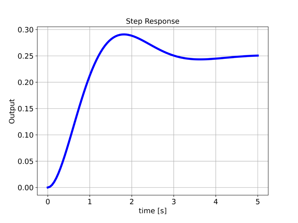
We can compute the step-response characteristics as follows:

# obtain the basic information about the step response
stepInfoData = ct.step_info(sysStateSpace)

This function will return this dictionary

{‘RiseTime’: 0.837303670179653,
‘SettlingTime’: 4.046967739201657,
‘SettlingMin’: 0.23487229056187914,
‘SettlingMax’: 0.2907583732260488,
‘Overshoot’: 16.303349290419522,
‘Undershoot’: 0,
‘Peak’: 0.2907583732260488,
‘PeakTime’: 1.814157952055915,
‘SteadyStateValue’: 0.25}

We can see that this function can be used to compute rise time, settling time, overshoot, peak time, etc.

We can compute the natural frequencies, damping ratios, and poles of the system as follows

ct.damp(sysStateSpace, doprint=True)

The result is

Eigenvalue_ Damping___ Frequency_
-1 +1.732j 0.5 2
-1 -1.732j 0.5 2
Out[119]: (array([2., 2.]), array([0.5, 0.5]), array([-1.+1.73205081j, -1.-1.73205081j]))

The poles are -1 +1.732j and -1 -1.732j . The damping ratio of these poles is 0.5 and the natural frequency is 2.

On the other hand, the poles and zeros can be computed as follows.

ct.poles(sysStateSpace)
ct.zeros(sysStateSpace)

The pole-zero map can be generalized as follows.

ct.pzmap(sysStateSpace)

Discretization of State-Space Models

We can discretize the state-space model as follows:

# discretization time
sampleTime=0.1
# discretize the system dynamics
# method='zoh' - zero order hold discretization
# method='bilinear' - bilinear discretization
sysStateSpaceDiscrete=ct.sample_system(sysStateSpace,sampleTime,method='zoh') 

# check if the system is in discrete-time
sysStateSpaceDiscrete.isdtime()

print(sysStateSpaceDiscrete)

# compute the step response

timeVector2=np.linspace(0,5,np.int32(np.floor(5/sampleTime)+1))
timeReturned2, systemOutput2 = ct.step_response(sysStateSpaceDiscrete,timeVector2)

# plot the step response
plottingFunction(timeReturned2,systemOutput2,titleString='Step Response',stringXaxis='time [s]' , stringYaxis='Output',stringFileName='stepResponse.png')

The function “sample_system()” is used to discretize the system. We specify the state-space model, sample time, and the discretization method. The function “isdtime()” is used to test if the system is discrete-time.