Python Control Systems Library Tutorial 1: Define Transfer Functions and Compute Step, Initial State, and Input Responses

In this control engineering and control theory tutorial, we provide an introduction to Python Control Systems Library. We explain how to

1. Install the library
2. Define transfer functions
3. Compute step response
4. Compute response to an arbitrary input
5. Compute the initial state response

The YouTube tutorial accompanying this webpage is given below.

The GitHub page with all the codes is given here.

Installation instructions

Here, we explain how to install the library. The basic installation is achieved by typing

pip install control

However, if you want to have the full functionality of this library, you need to perform the following

pip install slycot
pip install control

The slycot library is used in some functions for MIMO systems. However, you can use the basic functionality by only installing the control systems library with “pip install control”.

Plotting Function and Definition of Transfer Functions

First, we need to import the necessary libraries and functions

import matplotlib.pyplot as plt
import control as ct
import numpy as np

The Control Systems Library is imported by typing

import control as ct

It is a standard convention recommended by the creators of the library to import control library as “ct”.

Next, we create a plotting function:

def plottingFunction(xAxisVector,yAxisVector,titleString,stringXaxis,stringYaxis,stringFileName):
    plt.figure(figsize=(8,6))
    plt.plot(xAxisVector,yAxisVector, color='blue',linewidth=4)
    plt.title(titleString, fontsize=14)
    plt.xlabel(stringXaxis, fontsize=14)
    plt.ylabel(stringYaxis,fontsize=14)
    plt.tick_params(axis='both',which='major',labelsize=14)
    plt.grid(visible=True)
    plt.savefig(stringFileName,dpi=600)
    plt.show()    

This function will be used to plot the time responses of a transfer function and to save the generated graph to a file. It accepts

• “xAxisVector” – vector defining time points
• “yAxisVector,titleString” – vector defining step response
• “titleString” – title of the graph
• “stringXaxis” – label of the x-axis
• “stringYaxis” – label of the y-axis
• “stringFileName” – name of the file to be saved

Let us consider the following transfer function

(1)  

We define this transfer function as follows

# define a transfer function
num=[1]
den=[1,2,4]

W=ct.tf(num,den)
print(W)

The list “num” corresponds to the coefficients of the polynomial in the numerator. The list “den” corresponds to the coefficients of the polynomial in the denominator. Similarly to MATLAB, we use the function “tf()” to define the transfer function. The arguments of this function are lists “num” and “den” defining the coefficients in the numerator and denominator. Finally, we print the transfer function.

System Responses

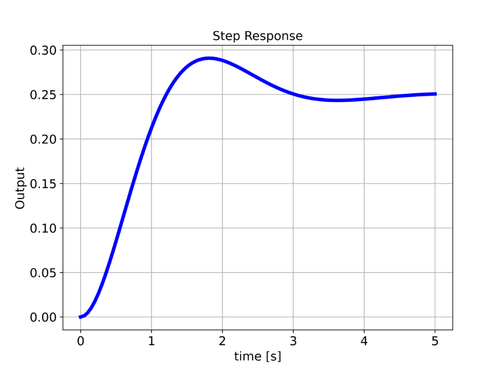
The step response is simulated like this.

###############################################################################
# simulate the step response
###############################################################################
timeVector=np.linspace(0,5,100)
timeReturned, systemOutput = ct.step_response(W,timeVector)

# plot the step response
plottingFunction(timeReturned,systemOutput,titleString='Step Response',stringXaxis='time [s]' , stringYaxis='Output',stringFileName='stepResponse.png')
###############################################################################

First, we define the time vector “timeVector”. Then, we call the function “step_response()” to compute the response. The first argument of this function is our transfer function W. The second argument is the time vector “timeVector”. The function returns the time used for simulation and the simulated output. By passing these arrays together with additional string arguments to “plottingFunction()”, we generate the graph given below.

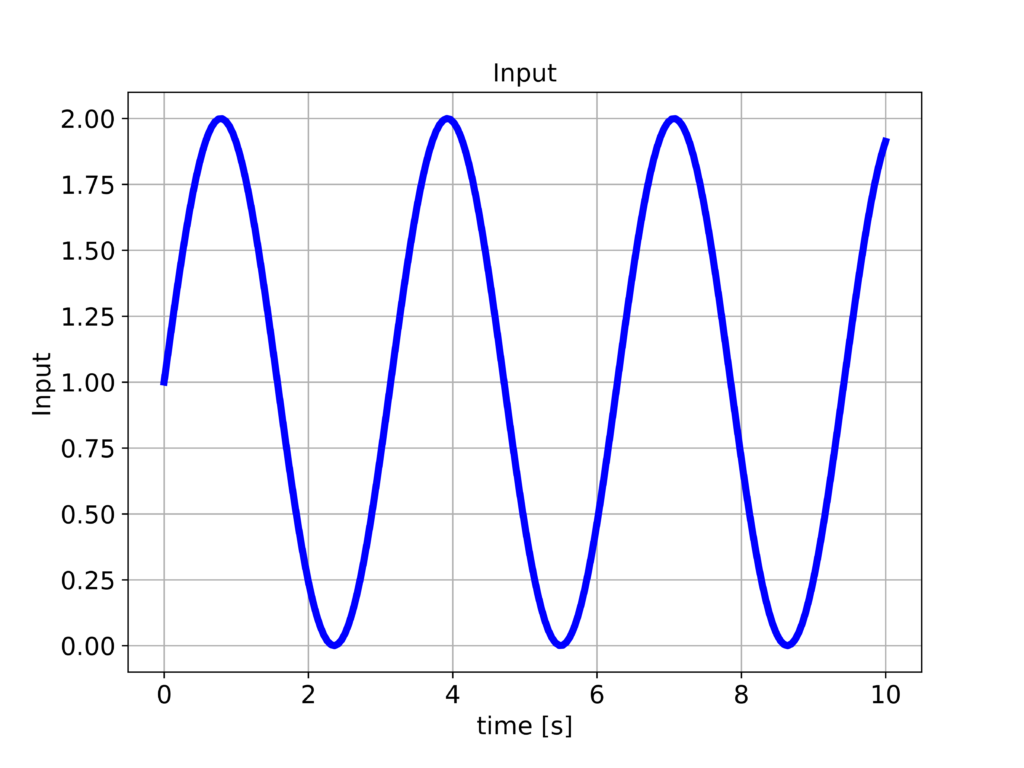
Next, we explain how to simulate the response of the system to arbitrary inputs. This is achieved by using the following code lines

###############################################################################
# Simulate the system response to a specific input
###############################################################################
# generate the input vector
timeVector2=np.linspace(0,10,200)
inputVector2=np.sin(2*timeVector2)+np.ones(timeVector2.shape)
# plot the input vector
plottingFunction(timeVector2,inputVector2,titleString='Input',stringXaxis='time [s]' , stringYaxis='Input', stringFileName='appliedInput.png')

# compute the response of the system to the specific input
timeReturned2, systemOutput2 = ct.forced_response(W,timeVector2,inputVector2)
plottingFunction(timeReturned2,systemOutput2,titleString='Sinusoidal output',stringXaxis='time [s]' , stringYaxis='Output', stringFileName='outputSinusoidal.png')
###############################################################################

We apply the input shown in the figure below to the system.

To simulate the response to this input, we use the function “forced_response()”. The first argument of this function is the transfer function. The second and third arguments are time and input vectors. The response of the system is given in the figure below.

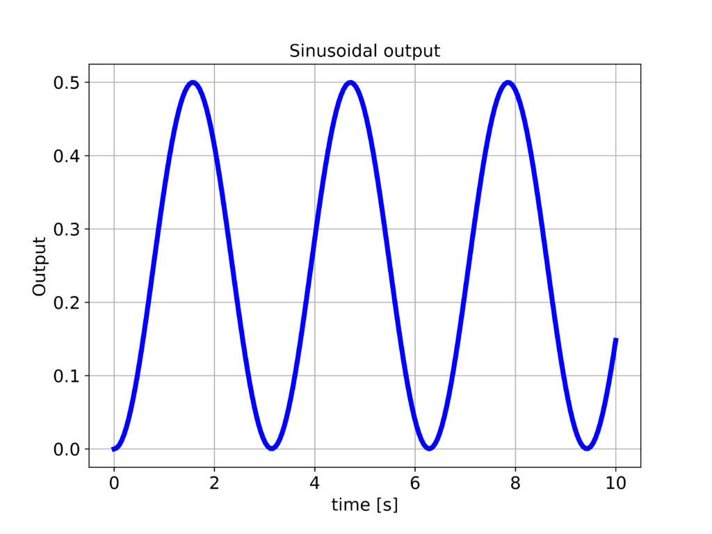
We can observe that the output is tracking the applied input. However, the output is attenuated. This is because of the 1/4 steady-state gain of the system.

Next, we explain how to simulate the response to non-zero initial states. We can do that by using the function “initial_response()” and the following code.

###############################################################################
# Simulate the system response to a non-zero input
# initial state response
###############################################################################
timeVector3=np.linspace(0,10,200)
initialState=np.array([2,-1])

timeReturned3, systemOutput3 = ct.initial_response(W,timeVector3,initialState)
plottingFunction(timeReturned3,systemOutput3,titleString='Initial state response',stringXaxis='time [s]' , stringYaxis='Output', stringFileName='outputInitial.png')

The initial state response is given in the figure below.

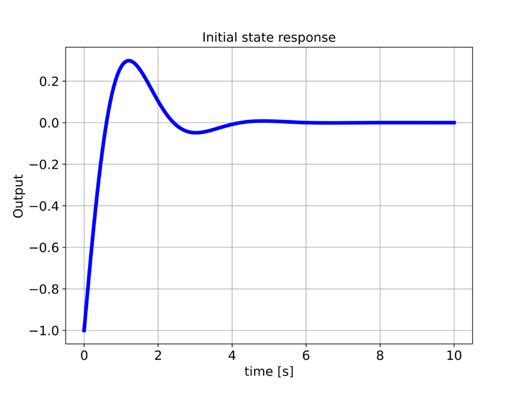
The system is asymptotically stable and consequently, the output of the system asymptotically approaches zero.