Simple and Easy-to-Understand Introduction to Recurrent Neural Networks for Time-Series Prediction in Keras and TensorFlow

In this post, we provide a brief and easy-to-understand introduction to recurrent neural networks for time series prediction. We use Keras and TensorFlow to implement the recurrent neural networks. The YouTube video accompanying this post is given below.

Often, people studying machine learning, as well as many machine learning practitioners who are afraid of mathematics, neglect basic mathematical equations underlying recurrent networks. However, to fully understand and know how to use recurrent neural networks, it is necessary to understand basic mathematics equations.

The simplest forms of recurrent neural networks are unsurprisingly called simple neural networks. The following equations mathematically describe recurrent neural networks:

(1)  

where

• is the hidden state vector at the time step
• is the input vector at the time step
• and are bias vectors that are trainable parameters
• A,B,C are matrices that are trainable parameters

The equation (1), defines the recurrent relationship:

(2)  

This relationship is illustrated in the figure below.

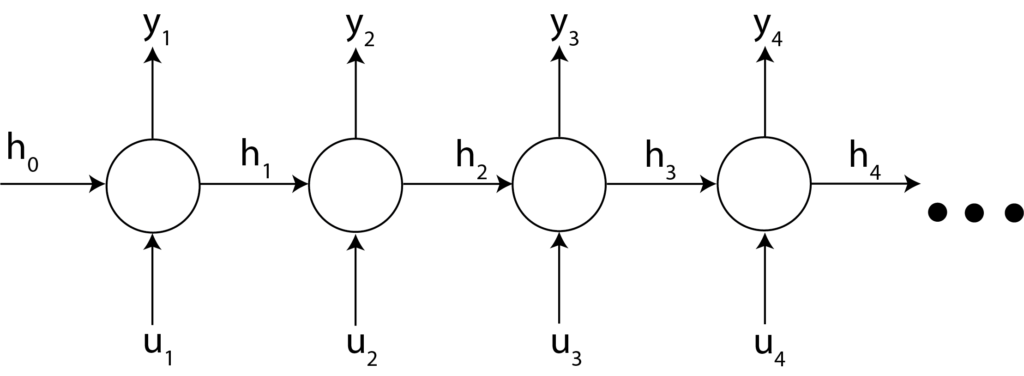
The network shown in Figure 1 is shown for the 4 time steps. The input sequence consists of inputs and and outputs and for the time steps .

There are also other recurrent networks with more complex mathematical forms than the form given by Eq. (1). Such networks are Long Short-Term Memory (LSTM) networks and Gated Recurrent Unit (GRU) networks. These network structures are designed to combat the vanishing gradient problem. However, the basic working principle of these networks is similar to the working principle of the simple recurrent networks.

Here, before we proceed with the explanation of the Python and Keras codes, we will explain one important detail. A typical code line that defines a recurrent neural network layer in Keras looks like this (see the code given later in the text for more details):

 keras.layers.GRU(5,return_sequences=True, use_bias=False, activation='linear', input_shape=[4,1])

Here, we should pay attention to one important input parameter. This parameter is “return_sequences=True”. According to the Keras documentation:

“return_sequences: Boolean. Whether to return the last output. in the output sequence, or the full sequence. Default: False.”

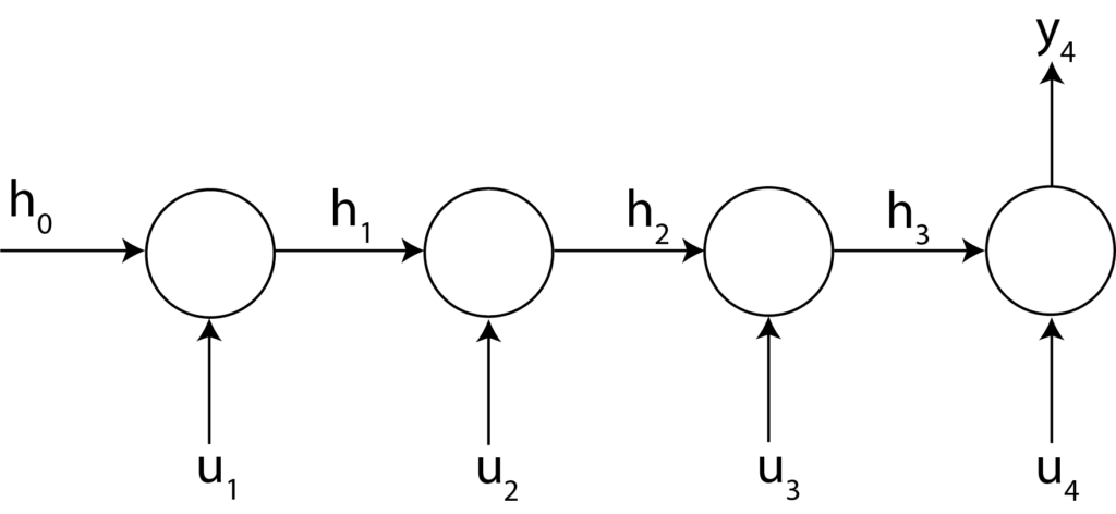
So, if we specify: “return_sequences=False”, we obtain the network structure shown in the figure below.

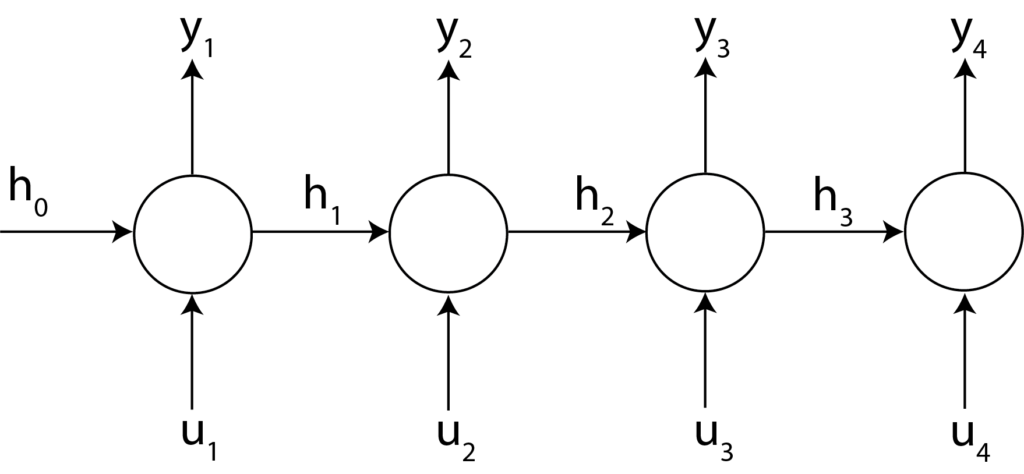
On the other hand, if we specify “return_sequences=True”, we obtain the network structure shown in the figure below.

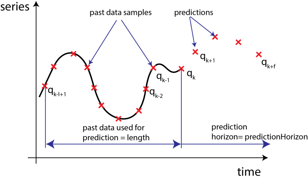
To explain the implementation of recurrent neural networks, we consider the problem of predicting time-series. The problem can be formulated as follows:

Let the time series samples be denoted by , where are discrete-time samples. At the time instant , given the current and past values of time series: , predict the future values of time series, given by .

The prediction problem is illustrated in the figure below.

There are several ways to solve this problem by using feedforward neural networks and recurrent neural networks. One approach is to use an encoder-decoder recurrent neural network structure. However, this approach might be a bit challenging to understand for beginners. We will explain this approach in our future posts and videos. Instead, we explain a simpler approach for time series prediction.

First, we import the necessary libraries and modules. Then we define the parameters and empty data sets. This is achieved by the following code lines.

# -*- coding: utf-8 -*-
"""
Created on Sat Jun 18 03:19:34 2022

@author: ahaber
"""
import numpy as np
import matplotlib.pyplot as plt
import tensorflow
from tensorflow import keras
from keras.callbacks import ModelCheckpoint

# total time steps for creating the function that needs to be learned
timeSteps=5000
# total number of samples for training, validation, and test
batchSize=200

# offset between two samples
offset=5
# past window
length=50
# prediction 
predictionHorizon=20

# create total empty data sets
# input data set
dataSetX=np.zeros(shape=(batchSize,length))
# output data set
dataSetY=np.zeros(shape=(batchSize,predictionHorizon))

We import numpy, pyplot, tensorflow, keras, and ModelCheckpoint libraries and modules. ModelCheckpoint is used to save the model weights during network training. This is necessary in order to find the model that produces the smallest validation error. Then, we specify the parameters timeSteps, batchSize, offset, length, and predictionHorizon. The meaning of these parameters will be explained later in the text. Next, we define the input data set “dataSetX” and output data set “dataSetY”.

Next, we create the time series (functions) that we want to predict.

# create the function that we want to learn
timeVector=np.linspace(0,50,timeSteps)
originalFunction=np.sin(50*0.6*timeVector+0.5)+np.sin(100*0.6*timeVector+0.5)+np.sin(100*0.05*timeVector+2)+0.01*np.random.randn(len(timeVector))   

# plot the function
plt.plot(originalFunction[0:100])
plt.xlabel('Time')
plt.ylabel('Function')
plt.savefig('function.png')
plt.show()

The function is shown in the figure below.

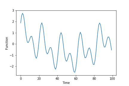
This function is a sum of sinusoidal signals of different frequencies and random noise. The parameter “timeSteps” determines the total number of time steps over which the function is defined. Next, by using the values of this function, we form the input “dataSetX” and output “dataSetY” data sets. The formation of these data sets is illustrated in the figure below.

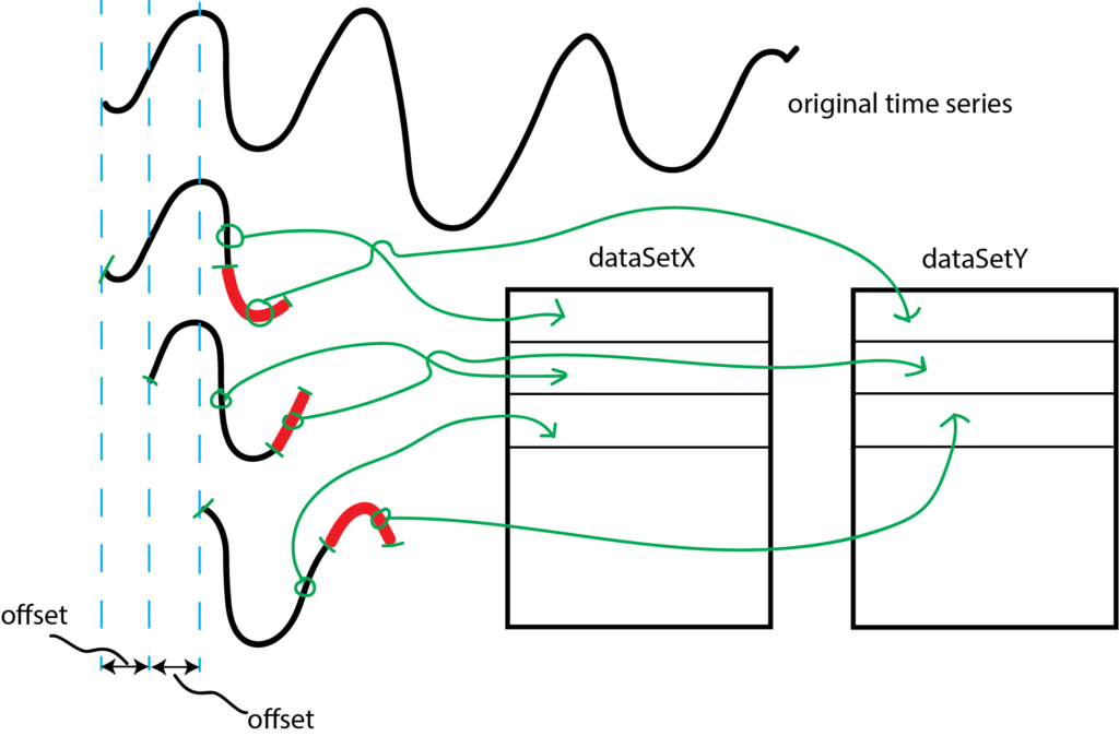
We form the input data set “dataSetX” as follows. The first row of the dataSetX consists of “0:length” samples (here we use the Numpy notation for range of samples, 0:length means that we take samples starting from 0 until length-1 sample). The corresponding first row of the output matrix consists of “length:(length+predictionHorizon)” samples. These samples are represented by the red color in Fig. 6. We are using the first “length” number of samples to predict the samples starting from “length+1” sample until “length+predictionHorizon” sample.

The second rows of the input and output matrices are formed in a similar manner, however, the samples are shifted by the value of “offset”. The following code lines are used to form the input and output matrices. At the end of the code, we reshape the data sets such that they are in the format that is appropriate for Keras recurrent neural network functions.

# create the data sets
for i in range(batchSize):
    dataSetX[i,:]=originalFunction[0+(i)*offset:length+(i)*offset]
    dataSetY[i,:]=originalFunction[length+(i)*offset:length+predictionHorizon+(i)*offset]

# reshape the data sets, such that we can use these data sets for recurrent neural networks
dataSetX=dataSetX.reshape((batchSize,length,1))
dataSetY=dataSetY.reshape((batchSize,predictionHorizon,1))

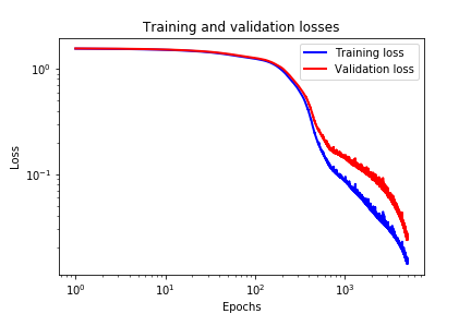
Next, we create three data sets: 1) training data set, 2) validation data set, and 3) test data set. Also, we create a neural network. The training data set is used to learn the parameters of the model. The validation data set is used during the training process. After every training epoch, the inputs from the validation data set are propagated through the trained model to create the predicted output. Together with the output from the validation data set, this predicted output is used to compute the validation loss. In this way, we can track the overfitting of the learning process. The overfitting process starts at the point at which the validation loss starts to increase, while the training loss is decreasing. We will save the model parameters that produce the smallest validation loss. In this way, we can prevent model overfitting. The following code lines are used to create the data sets and create the neural network.

# create train, validation, and test data sets
Xtrain, Ytrain = dataSetX[:(int)(0.6*batchSize),:], dataSetY[:(int)(0.6*batchSize),:]
Xvalid, Yvalid = dataSetX[(int)(0.6*batchSize):(int)(0.8*batchSize),:], dataSetY[(int)(0.6*batchSize):(int)(0.8*batchSize),:]
Xtest, Ytest = dataSetX[(int)(0.8*batchSize):,:], dataSetY[(int)(0.8*batchSize):,:]   

# create the model
model= keras.models.Sequential([keras.layers.GRU(5,return_sequences=True, use_bias=False, activation='linear', input_shape=[None,1]),keras.layers.GRU(5,return_sequences=False, use_bias=False, activation='linear'), keras.layers.Dense(predictionHorizon,activation='linear')])

We use the Gated Recurrent Unit networks. We use two layers of GRUs with one final dense layer. The dense layer has “predictionHorizon” neurons. That is, the number of neurons is equal to the number of prediction steps. In the first GRU layer, we specify “return_sequences=True”. This structure is illustrated in Fig. 3.

Next, we create the model checkpoint for saving model parameters that produce the lowest validation loss. Then, we compile the model by using mean squared error as the loss and the optimizer. After that, we fit the model. In every epoch, the model parameters are saved that produce the lowest validation loss. After the fitting process is completed, we load the weights that produce the lowest validation error. Finally, we use the test data set to predict the model ouputs. These steps are performed by executing the following code lines

# create a model check point
# C:\codes\recursive\saved_models\
#filepath="\\codes\\recursive\\saved_models\\weights-{epoch:02d}-{val_loss:.6f}.hdf5"
filepath="\\codes\\recursive\\saved_models\\weights.hdf5"
checkpoint = ModelCheckpoint(filepath, monitor='val_loss', verbose=0, save_best_only=True, save_weights_only=False, mode='auto')
callbacks_list = [checkpoint]

# compile the model    
model.compile(loss="mean_squared_error", optimizer="adam", metrics=['mse'])
model.summary()
# fit the model
history= model.fit(Xtrain, Ytrain, batch_size=100, epochs=5000, validation_data=(Xvalid, Yvalid),callbacks=callbacks_list,verbose=2)
# load weights
model.load_weights("\\codes\\recursive\\saved_models\\weights.hdf5")

# predict
prediction = model.predict(Xtest)

Next, we plot the validation and training losses:

# plot the training and validation curves
loss=history.history['loss']
val_loss=history.history['val_loss']
epochs=range(1,len(loss)+1)
plt.figure()
plt.plot(epochs, loss,'b', label='Training loss',linewidth=2)
plt.plot(epochs, val_loss,'r', label='Validation loss',linewidth=2)
plt.title('Training and validation losses')
plt.xlabel('Epochs')
plt.ylabel('Loss')
plt.xscale('log')
plt.yscale('log')
plt.legend()
plt.savefig('validation_and_loss.png')
plt.show()

These losses are shown in the figure below.

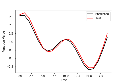
Finally, we plot the prediction performance of the network evaluated on the training data set. The prediction graphs are generate by using the following code lines.

# visualize the prediction and test data
plt.plot(prediction[1,:],color='k',label='Predicted',linewidth=2)
plt.plot(Ytest[1,:],color='r',label='Test',linewidth=2)
plt.xlabel('Time')
plt.ylabel('Function Value')
plt.legend()
plt.savefig('prediction1.png')
plt.show()

# visualize the prediction and test data
plt.plot(prediction[2,:],color='k',label='Predicted',linewidth=2)
plt.plot(Ytest[2,:],color='r',label='Test',linewidth=2)
plt.xlabel('Time')
plt.ylabel('Function Value')
plt.legend()
plt.savefig('prediction2.png')
plt.show()

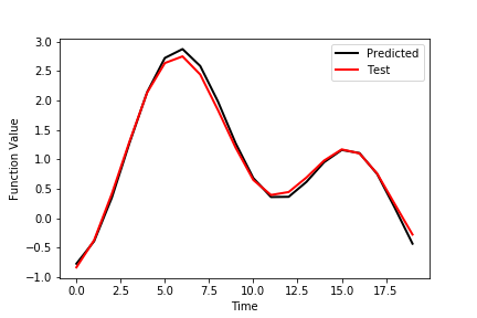
The figure below shows the outputs of the first row of the test data set as well as the predicted outputs.

The figure below shows the outputs of the second row of the test data set as well as the predicted outputs.