Deep Q Networks (DQN) in Python From Scratch by Using OpenAI Gym and TensorFlow- Reinforcement Learning Tutorial – Fusion of Engineering, Control, Coding, Machine Learning, and Science

In this reinforcement learning tutorial, we explain how to implement the Deep Q Network (DQN) algorithm in Python from scratch by using the OpenAI Gym and TensorFlow machine learning libraries. The GitHub page with all the codes is given here. The YouTube videos accompanying this post are given below.

Basic Concepts of Deep Q Networks

Before reading this tutorial, it is a good idea to obtain enough preliminary knowledge that will enable you to understand the material presented in this tutorial. To be able to understand this tutorial, you need to understand these two topics:

In the sequel, we provide a brief explanation of the main concepts related to the implementation of the DQN algorithm.

First, let us motivate the need for introducing neural networks in reinforcement learning algorithms, and in particular, in the Q-learning algorithm. The “classical” Q-learning method based on keeping a table of action value functions Q is memory-consuming and becomes infeasible when the state-space dimension increases. Even for the 4-dimensional state space of the cart-pole system, the table storing the Q value functions for different states becomes extremely large and difficult to accurately estimate. Can we somehow modify the Q-learning algorithm such that we do not need to store all the action value function values for different states? In principle, the answer is YES. The idea is to estimate a function that will produce the action value function values for a given state. That is, we want to directly learn this function or a map that will transform input states into action value function values. For example, let us consider the Cart Pole OpenAI Gym environment, shown in the figure below.

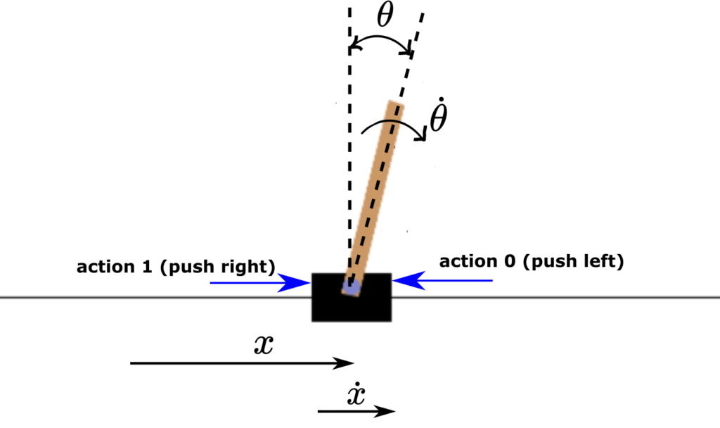
Figure 1: Cart-Pole OpenAI Gym Environment.

This system has four states: position of the cart $x$ , velocity of the cart $\dot{x}$ , pole angular rotation $\theta$ , and pole angular velocity $\dot{\theta}$ . We have two actions: push the cart left (action 0) and push the cart right (action 1). The control objective is to find a sequence of control actions that will keep the pendulum in the vertical position.

For that purpose, we want to estimate (or in machine learning terms – to learn) a function that maps the state vector $S=[x,\dot{x},\theta,\dot{\theta}]^{T}$ into action value functions for this particular state. That is, we want to estimate this mapping.

(1) $\begin{align*}\begin{bmatrix}Q(S,A=0) \\ Q(S,A=1) \end{bmatrix}=F\Big(S=\begin{bmatrix} x \\ \dot{x} \\ \theta \\ \dot{\theta}\end{bmatrix} \Big) \end{align*}$

Where $F$ is a mapping that we want to estimate or in other words to learn. That is, for a given state $S$ , $F$ is a map (nonlinear in the general case) that produces two values of the action value functions obtained for the particular actions $A=0$ (push the cart left) and $A=1$ (push the cart right).

The main idea of the deep Q networks is to use a neural network as the mapping $F$ . This is shown in the figure below.

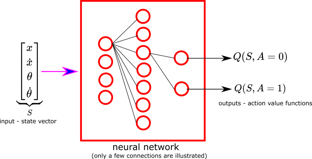
Figure 2: Neural network for approximating the action value functions.

Our goal will be to train this network. Once we train this network, we will use its prediction and the greedy approach to select the optimal control actions.

To train the network, we need to introduce the concept of the replay buffer or replay memory (this concept is also known as the experienced replay). In the sequel, we explain this important concept.

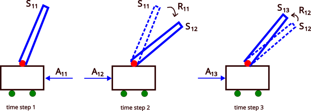
Consider a sequence of states and actions of the cart pole system shown in Fig. 3 below. Let an initial state in the episode 1, be denoted by $S_{11}$ . Then, let us say that we somehow determine a control action $A_{11}$ , and apply it to the environment. We obtain the reward $R_{11}$ , and the environment evolves to the next state $S_{12}$ . Then, we repeat this procedure in the state $S_{12}$ . We compute the action $A_{12}$ , we apply it to the environment in order to obtain the reward $R_{12}$ while the environment evolves to the state $S_{13}$ . We repeat this procedure until the end of the episode. Let us say that episode has $N_{1}$ time-steps. The terminal state is then $S_{1N_{1}}$ .

Figure 3: Illustration of the state transitions.

Next, we start the second episode. Let the initial state be denoted by $S_{21}$ . Then, we compute the action $A_{21}$ and apply it to the environment. This action produces the reward $R_{21}$ , and the environment evolves to the state $S_{22}$ . Then, in the state $S_{22}$ , we repeat this procedure until we reach the terminal state $S_{2N_{2}}$ (we assume that the episode has $N_{2}$ time-steps). In the third, fourth, etc., episodes we repeat the same procedure. We store the obtained data in a replay buffer that is illustrated in the figure below.

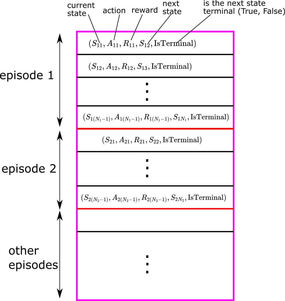
Figure 4: Illustration of the replay buffer

To create the replay buffer, we store the current state, action in the current state, reward, next state, and the boolean variable “IsTerminal” in a tuple. The boolean variable “IsTerminal” denotes if the next state is a terminal state (YES) or not (FALSE). We store the tuples on top of each other until the end of the episode. Then, we repeat this procedure for a certain number of episodes. In this way, we obtain states, rewards, and actions for a number of episodes. We use the queue data structure to implement this replay buffer. That is, let us say that this buffer has $N$ cells for recording the tuples. Then, let us say that a new tuple is recorded $(S_{ij},A_{ij},R_{ij},S_{i(j+1)},\text{IsTerminal})$ , then we add this tuple at the end of the queue, and at the same time, we remove the first tuple from the queue. In this way, we obtain $N$ recent data tuples.

When training the network, we do not use the full replay buffer (full batch of data). Instead, we randomly select tuples from the batch, and we form a new batch that is used for training. This is illustrated in the figure below.

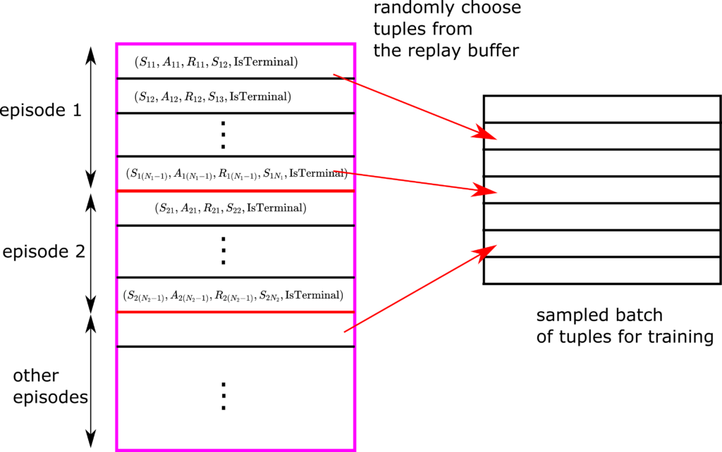
Figure 5: Random sampling from the replay buffer to form a batch of data for training.

This is done since the states in the subsequent tuples in the replay buffer might be highly correlated. Consequently, subsequent tuples might not carry significant new information with respect to each other, and this implies a slow learning process. To improve the speed of the learning process, we randomly sample tuples and form a new batch of tuples that are less mutually correlated. In this way, we speed up the learning process.

While training the Q learning model, we actually have two networks.

Online network. We call this network also the main network in the code that is presented in the second part of this tutorial. This is the network that we constantly update during the training process. This is the reason why we call this network the online network. Also, this network is used to predict the action value functions, and once the training process is completed, this network is used to form the greedy policy. Let the predictions performed by this network be denoted by

(2) $\begin{align*}\text{Online network action value prediction:}\;\;\; Q(S,A,\theta)\end{align*}$

where $\theta$ is the vector of the parameters of the neural network. The training algorithm constantly updates $\theta$ .

Target network. This network is used to compute the target output samples for training the network. That is, the predictions performed by this network, as well as obtained rewards, are used to form the outputs for the training process. This network is also updated. That is, its parameters are also updated. However, the parameters are updated less frequently than the online network. For example, we update this network every 100-time steps (can also be a much larger number). The action value function values predicted by this network are denoted by

(3) $\begin{align*}\text{Target network action value prediction:} \;\;\; Q(S,A,\tilde{\theta})\end{align*}$

At the beginning of the training process, we set $\tilde{\theta}\leftarrow \theta$ . That is, both online and target networks are the same. Then, after a certain number of time steps (for example after 100 or more time steps), we again set $\tilde{\theta}\leftarrow \theta$ (we copy the parameters from the online to the target network).

Now, that we have a basic understanding of the target and online networks, we need to define the cost function.

We aim at minimizing the following cost function

(4) $\begin{align*}\frac{1}{N} \sum_{i=1}^{N} \Big( y_{i} - Q(S_{i},A_{i},\theta) \Big)^{2} \end{align*}$

where if the next state $S_{i}^{'}$ IS NOT the terminal state:

(5) $\begin{align*}& y_{i}=R_{i}+\gamma Q_{\text{max}}(S_{i}^{'},\tilde{\theta}) \\& Q_{\text{max}}(S_{i}^{'})=\text{max}_{A} Q(S_{i}^{'},A,\tilde{\theta})\end{align*}$

and if the next state $S_{i}^{'}$ IS the terminal state:

(6) $\begin{align*}y_{i}=R_{i}\end{align*}$

Here, we need to introduce a few important explanations, such that we can successfully implement the learning process. The number $N$ is the total number of tuples in the training data batch used to form the cost function. We form a single entry in the above sum by using the tuple $(S_{i},A_{i},R_{i},S_{i}^{'},\text{IsTerminal})$ from the training batch. Here $S_{i}$ is the current state, $A_{i}$ is the action in the state $S_{i}$ , $R_{i}$ is the obtained reward, and $S_{i}^{'}$ is the next state that is produced by applying the action $A_{i}$ . The parameter $\gamma$ is the discount rate. The value of $y_{i}$ is a real number that is the target output. The input is the state $S_{i}$ . If the next state $S_{i}^{'}$ is not a terminal state, then we compute $y_{i}$ by using

(7) $\begin{align*}& y_{i}=R_{i}+\gamma Q_{\text{max}}(S_{i}^{'},\tilde{\theta}) \\& Q_{\text{max}}(S_{i}^{'})=\text{max}_{A} Q(S_{i}^{'},A,\tilde{\theta})\end{align*}$

where the value $Q_{\text{max}}(S_{i}^{'},\tilde{\theta})$ is computed by using the target network. To compute this value, we simply put an input $S_{i}^{'}$ to the target network and produce the predictions $Q(S_{i}^{'},A=0,\tilde{\theta})$ and $Q(S_{i}^{'},A=1,\tilde{\theta})$ by forward propagating $S_{i}^{'}$ through the target network. Then $Q_{\text{max}}(S_{i}^{'},\tilde{\theta})$ is simply a maximum of these two predictions.

Now, we are ready to summarize the deep Q-learning network algorithm.

Summary of the Deep Q Learning Network Reinforcement Learning Algorithm

First, we explain the main preliminary steps. There are also some other steps that are related to the choice of the parameters or network structure. To keep this tutorial relatively short, we only mention the main preliminary steps:

Preliminary steps:

Create a general form of the online network. Note that the target network should have the same structure as the online network.
Initialize the vector of parameters $\theta$ of the online network.
Set $\tilde{\theta}\leftarrow \theta$ . That is, copy the parameters of the online network to the target network.

Loop through training episodes:

STEP 1: Initialize the environment and observe the initial state. Here we reset the environment, such that we erase traces from the previous episode’s simulation. We set the current state to be the initial state.

STEP 2: Loop through the time steps of the current episode. That is, loop through the time steps until the next state is the terminal state. For every time step perform this:

STEP 2.1: In the current state, select the control action $A$ . We use the epsilon greedy approach for selecting the actions. Note that during the first several episodes we can completely randomly select the control actions since we do not have enough data. Also, note that we use the current version of the online network to produce action value functions for selecting epsilon-greedy actions.

STEP 2.2:
– Apply the control actions to the environment, and observe the reward and the next state.
– Append the tuple (current state, action, reward, next state, “IsTerminal”) to the replay buffer.

STEP 2.3: Train the online network and if the right conditions are met, update the target network. If the number of tuples in the replay buffer is smaller than the maximal length of the replay buffer, then skip this step (go to the step 2.4). If the replay buffer is full, then proceed with this step.
– Sample a training batch from the replay buffer (that is, choose a predefined number of random tuple samples from the replay buffer).
– Create samples of input and output data necessary to form the cost function (4).
– Train the online network starting from initial vector parameters $\theta$ from the previous time step.
– If a certain number of time steps has passed (for example, 100 of time steps), perform the following assignment: $\tilde{\theta}\leftarrow \theta$ . That is, we copy the parameters from the online network to the target network. Here, the time samples for updating the target network parameters can span several episodes.

STEP 2.4: Set the current state to the next state, and go to the STEP 2.1. If the next state is the terminal state, the loop that simulates time-steps in an episode completes, and the new episode starts. In that case, we go to STEP 1.

Once we have learned the parameters of the online network (after many episodes), at every time step of the test episode, we create an optimal policy by predicting the Q values for the current state (this is done by forward propagation of the online network), and simply selecting an action to apply that maximizes the predicted Q values at the current state. That is, we use the greedy approach for selecting the optimal policy.

Python and TensorFlow implementation of the Deep Q Network Learning Algorithm

We use an object-oriented approach to implement the DQN learning algorithm. In the sequel, we give a complete class definition, and then, we explain its main parts. All the codes are posted on the GitHub page which can be found here. The class is given below.

# import the necessary libraries
import numpy as np
import random
from tensorflow.keras.layers import Dense
from tensorflow.keras.models import Sequential
from tensorflow.keras.optimizers import RMSprop
from collections import deque 
from tensorflow import gather_nd
from tensorflow.keras.losses import mean_squared_error 



class DeepQLearning:
    
    ###########################################################################
    #   START - __init__ function
    ###########################################################################
    # INPUTS: 
    # env - Cart Pole environment
    # gamma - discount rate
    # epsilon - parameter for epsilon-greedy approach
    # numberEpisodes - total number of simulation episodes
    
            
    def __init__(self,env,gamma,epsilon,numberEpisodes):
        
        
        self.env=env
        self.gamma=gamma
        self.epsilon=epsilon
        self.numberEpisodes=numberEpisodes
        
        # state dimension
        self.stateDimension=4
        # action dimension
        self.actionDimension=2
        # this is the maximum size of the replay buffer
        self.replayBufferSize=300
        # this is the size of the training batch that is randomly sampled from the replay buffer
        self.batchReplayBufferSize=100
        
        # number of training episodes it takes to update the target network parameters
        # that is, every updateTargetNetworkPeriod we update the target network parameters
        self.updateTargetNetworkPeriod=100
        
        # this is the counter for updating the target network 
        # if this counter exceeds (updateTargetNetworkPeriod-1) we update the network 
        # parameters and reset the counter to zero, this process is repeated until the end of the training process
        self.counterUpdateTargetNetwork=0
        
        # this sum is used to store the sum of rewards obtained during each training episode
        self.sumRewardsEpisode=[]
        
        # replay buffer
        self.replayBuffer=deque(maxlen=self.replayBufferSize)
        
        # this is the main network
        # create network
        self.mainNetwork=self.createNetwork()
        
        # this is the target network
        # create network
        self.targetNetwork=self.createNetwork()
        
        # copy the initial weights to targetNetwork
        self.targetNetwork.set_weights(self.mainNetwork.get_weights())
        
        # this list is used in the cost function to select certain entries of the 
        # predicted and true sample matrices in order to form the loss
        self.actionsAppend=[]
    
    ###########################################################################
    #   END - __init__ function
    ###########################################################################
    
    ###########################################################################
    # START - function for defining the loss (cost) function
    # INPUTS: 
    #
    # y_true - matrix of dimension (self.batchReplayBufferSize,2) - this is the target 
    # y_pred - matrix of dimension (self.batchReplayBufferSize,2) - this is predicted by the network
    # 
    # - this function will select certain row entries from y_true and y_pred to form the output 
    # the selection is performed on the basis of the action indices in the list  self.actionsAppend
    # - this function is used in createNetwork(self) to create the network
    #
    # OUTPUT: 
    #    
    # - loss - watch out here, this is a vector of (self.batchReplayBufferSize,1), 
    # with each entry being the squared error between the entries of y_true and y_pred
    # later on, the tensor flow will compute the scalar out of this vector (mean squared error)
    ###########################################################################    
    
    def my_loss_fn(self,y_true, y_pred):
        
        s1,s2=y_true.shape
        #print(s1,s2)
        
        # this matrix defines indices of a set of entries that we want to 
        # extract from y_true and y_pred
        # s2=2
        # s1=self.batchReplayBufferSize
        indices=np.zeros(shape=(s1,s2))
        indices[:,0]=np.arange(s1)
        indices[:,1]=self.actionsAppend
        
        # gather_nd and mean_squared_error are TensorFlow functions
        loss = mean_squared_error(gather_nd(y_true,indices=indices.astype(int)), gather_nd(y_pred,indices=indices.astype(int)))
        #print(loss)
        return loss    
    ###########################################################################
    #   END - of function my_loss_fn
    ###########################################################################
    
    
    ###########################################################################
    #   START - function createNetwork()
    # this function creates the network
    ###########################################################################
    
    # create a neural network
    def createNetwork(self):
        model=Sequential()
        model.add(Dense(128,input_dim=self.stateDimension,activation='relu'))
        model.add(Dense(56,activation='relu'))
        model.add(Dense(self.actionDimension,activation='linear'))
        # compile the network with the custom loss defined in my_loss_fn
        model.compile(optimizer = RMSprop(), loss = self.my_loss_fn, metrics = ['accuracy'])
        return model
    ###########################################################################
    #   END - function createNetwork()
    ###########################################################################
            
    ###########################################################################
    #   START - function trainingEpisodes()
    #   - this function simulates the episodes and calls the training function 
    #   - trainNetwork()
    ###########################################################################

    def trainingEpisodes(self):
   
        
        # here we loop through the episodes
        for indexEpisode in range(self.numberEpisodes):
            
            # list that stores rewards per episode - this is necessary for keeping track of convergence 
            rewardsEpisode=[]
                       
            print("Simulating episode {}".format(indexEpisode))
            
            # reset the environment at the beginning of every episode
            (currentState,_)=self.env.reset()
                      
            # here we step from one state to another
            # this will loop until a terminal state is reached
            terminalState=False
            while not terminalState:
                                      
                # select an action on the basis of the current state, denoted by currentState
                action = self.selectAction(currentState,indexEpisode)
                
                # here we step and return the state, reward, and boolean denoting if the state is a terminal state
                (nextState, reward, terminalState,_,_) = self.env.step(action)          
                rewardsEpisode.append(reward)
         
                # add current state, action, reward, next state, and terminal flag to the replay buffer
                self.replayBuffer.append((currentState,action,reward,nextState,terminalState))
                
                # train network
                self.trainNetwork()
                
                # set the current state for the next step
                currentState=nextState
            
            print("Sum of rewards {}".format(np.sum(rewardsEpisode)))        
            self.sumRewardsEpisode.append(np.sum(rewardsEpisode))
    ###########################################################################
    #   END - function trainingEpisodes()
    ###########################################################################
            
       
    ###########################################################################
    #    START - function for selecting an action: epsilon-greedy approach
    ###########################################################################
    # this function selects an action on the basis of the current state 
    # INPUTS: 
    # state - state for which to compute the action
    # index - index of the current episode
    def selectAction(self,state,index):
        import numpy as np
        
        # first index episodes we select completely random actions to have enough exploration
        # change this
        if index<1:
            return np.random.choice(self.actionDimension)   
            
        # Returns a random real number in the half-open interval [0.0, 1.0)
        # this number is used for the epsilon greedy approach
        randomNumber=np.random.random()
        
        # after index episodes, we slowly start to decrease the epsilon parameter
        if index>200:
            self.epsilon=0.999*self.epsilon
        
        # if this condition is satisfied, we are exploring, that is, we select random actions
        if randomNumber < self.epsilon:
            # returns a random action selected from: 0,1,...,actionNumber-1
            return np.random.choice(self.actionDimension)            
        
        # otherwise, we are selecting greedy actions
        else:
            # we return the index where Qvalues[state,:] has the max value
            # that is, since the index denotes an action, we select greedy actions
                       
            Qvalues=self.mainNetwork.predict(state.reshape(1,4))
          
            return np.random.choice(np.where(Qvalues[0,:]==np.max(Qvalues[0,:]))[0])
            # here we need to return the minimum index since it can happen
            # that there are several identical maximal entries, for example 
            # import numpy as np
            # a=[0,1,1,0]
            # np.where(a==np.max(a))
            # this will return [1,2], but we only need a single index
            # that is why we need to have np.random.choice(np.where(a==np.max(a))[0])
            # note that zero has to be added here since np.where() returns a tuple
    ###########################################################################
    #    END - function selecting an action: epsilon-greedy approach
    ###########################################################################
    
    ###########################################################################
    #    START - function trainNetwork() - this function trains the network
    ###########################################################################
    
    def trainNetwork(self):

        # if the replay buffer has at least batchReplayBufferSize elements,
        # then train the model 
        # otherwise wait until the size of the elements exceeds batchReplayBufferSize
        if (len(self.replayBuffer)>self.batchReplayBufferSize):
            

            # sample a batch from the replay buffer
            randomSampleBatch=random.sample(self.replayBuffer, self.batchReplayBufferSize)
            
            # here we form current state batch 
            # and next state batch
            # they are used as inputs for prediction
            currentStateBatch=np.zeros(shape=(self.batchReplayBufferSize,4))
            nextStateBatch=np.zeros(shape=(self.batchReplayBufferSize,4))            
            # this will enumerate the tuple entries of the randomSampleBatch
            # index will loop through the number of tuples
            for index,tupleS in enumerate(randomSampleBatch):
                # first entry of the tuple is the current state
                currentStateBatch[index,:]=tupleS[0]
                # fourth entry of the tuple is the next state
                nextStateBatch[index,:]=tupleS[3]
            
            # here, use the target network to predict Q-values 
            QnextStateTargetNetwork=self.targetNetwork.predict(nextStateBatch)
            # here, use the main network to predict Q-values 
            QcurrentStateMainNetwork=self.mainNetwork.predict(currentStateBatch)
            
            # now, we form batches for training
            # input for training
            inputNetwork=currentStateBatch
            # output for training
            outputNetwork=np.zeros(shape=(self.batchReplayBufferSize,2))
            
            # this list will contain the actions that are selected from the batch 
            # this list is used in my_loss_fn to define the loss-function
            self.actionsAppend=[]            
            for index,(currentState,action,reward,nextState,terminated) in enumerate(randomSampleBatch):
                
                # if the next state is the terminal state
                if terminated:
                    y=reward                  
                # if the next state if not the terminal state    
                else:
                    y=reward+self.gamma*np.max(QnextStateTargetNetwork[index])
                
                # this is necessary for defining the cost function
                self.actionsAppend.append(action)
                
                # this actually does not matter since we do not use all the entries in the cost function
                outputNetwork[index]=QcurrentStateMainNetwork[index]
                # this is what matters
                outputNetwork[index,action]=y
            
            # here, we train the network
            self.mainNetwork.fit(inputNetwork,outputNetwork,batch_size = self.batchReplayBufferSize, verbose=0,epochs=100)     
            
            # after updateTargetNetworkPeriod training sessions, update the coefficients 
            # of the target network
            # increase the counter for training the target network
            self.counterUpdateTargetNetwork+=1  
            if (self.counterUpdateTargetNetwork>(self.updateTargetNetworkPeriod-1)):
                # copy the weights to targetNetwork
                self.targetNetwork.set_weights(self.mainNetwork.get_weights())        
                print("Target network updated!")
                print("Counter value {}".format(self.counterUpdateTargetNetwork))
                # reset the counter
                self.counterUpdateTargetNetwork=0
    ###########################################################################
    #    END - function trainNetwork() 
    ###########################################################################

First, we explain “__init__()” function that is given below.

 def __init__(self,env,gamma,epsilon,numberEpisodes):
        
        
        self.env=env
        self.gamma=gamma
        self.epsilon=epsilon
        self.numberEpisodes=numberEpisodes
        
        # state dimension
        self.stateDimension=4
        # action dimension
        self.actionDimension=2
        # this is the maximum size of the replay buffer
        self.replayBufferSize=300
        # this is the size of the training batch that is randomly sampled from the replay buffer
        self.batchReplayBufferSize=100
        
        # number of training episodes it takes to update the target network parameters
        # that is, every updateTargetNetworkPeriod we update the target network parameters
        self.updateTargetNetworkPeriod=100
        
        # this is the counter for updating the target network 
        # if this counter exceeds (updateTargetNetworkPeriod-1) we update the network 
        # parameters and reset the counter to zero, this process is repeated until the end of the training process
        self.counterUpdateTargetNetwork=0
        
        # this sum is used to store the sum of rewards obtained during each training episode
        self.sumRewardsEpisode=[]
        
        # replay buffer
        self.replayBuffer=deque(maxlen=self.replayBufferSize)
        
        # this is the main network
        # create network
        self.mainNetwork=self.createNetwork()
        
        # this is the target network
        # create network
        self.targetNetwork=self.createNetwork()
        
        # copy the initial weights to targetNetwork
        self.targetNetwork.set_weights(self.mainNetwork.get_weights())
        
        # this list is used in the cost function to select certain entries of the 
        # predicted and true sample matrices in order to form the loss
        self.actionsAppend=[]

The inputs are:

“env” – Cart Pole environment
“gamma” – discount rate
“epsilon” – epsilon parameter for epsilon-greedy approach
“numberEpisodes” – total number of simulation episodes

Next, we set the following parameters:

“self.stateDimension=4” – this is the state dimension
“self.actionDimension=2” – this is the action dimension
“self.replayBufferSize=300” – this is the size of the replay buffer. We are basically saying that we want a buffer that will store 300 tuples.
“self.batchReplayBufferSize=100” – this is the size of the batch of tuples that is sampled from “self.replayBufferSize”. This is done in STEP 2.3 of the DQN learning algorithm.
“self.updateTargetNetworkPeriod=100” – this parameter is used to denote how frequently (in terms of time steps), we update the target network. In our case, it is 100 time steps, however, you can increase or decrease this parameter (it is a tuning factor).
“self.counterUpdateTargetNetwork=0” – this counter goes from 0 to “self.updateTargetNetworkPeriod”. When it reaches the final value, we update the target network.
“self.sumRewardsEpisode=[]” – this list is used to store the sum of rewards obtained during each training episode. We quantify the convergence of the training process by analyzing the sum of rewards.
“self.replayBuffer=deque(maxlen=self.replayBufferSize)” – this is the replay buffer.
“self.mainNetwork=self.createNetwork()” – this code line will call the function “createNetwork()”, and it will return the online network. We will explain “createNetwork()” function in the sequel.
“self.targetNetwork=self.createNetwork()” – this will create the target network with the same structure as the online network.
“self.targetNetwork.set_weights(self.mainNetwork.get_weights())” – here we copy the weights from the online network to the target network.
“self.actionsAppend=[]” – this list is used to store actions for forming the batch of data. It is used in the function “self.my_loss_fn()” to define the cost function for optimization

Next, we discuss the function used to define the network. The code is given below.

 # create a neural network
    def createNetwork(self):
        model=Sequential()
        model.add(Dense(128,input_dim=self.stateDimension,activation='relu'))
        model.add(Dense(56,activation='relu'))
        model.add(Dense(self.actionDimension,activation='linear'))
        # compile the network with the custom loss defined in my_loss_fn
        model.compile(optimizer = RMSprop(), loss = self.my_loss_fn, metrics = ['accuracy'])
        return model

This code is self-explanatory. We create a sequential natural network. The most important part to observe is that we tell to TensorFlow that we have defined a custom loss-function. We do that in the model.compile() function, by specifying “loss = self.my_loss_fn”.

The cost function is defined below.

 def my_loss_fn(self,y_true, y_pred):
        
        s1,s2=y_true.shape
        #print(s1,s2)
        
        # this matrix defines indices of a set of entries that we want to 
        # extract from y_true and y_pred
        # s2=2
        # s1=self.batchReplayBufferSize
        indices=np.zeros(shape=(s1,s2))
        indices[:,0]=np.arange(s1)
        indices[:,1]=self.actionsAppend
        
        # gather_nd and mean_squared_error are TensorFlow functions
        loss = mean_squared_error(gather_nd(y_true,indices=indices.astype(int)), gather_nd(y_pred,indices=indices.astype(int)))
        #print(loss)
        return loss

Here, a few important things should be mentioned. This function takes two input parameters “y_true” and “y_pred”. Both of these inputs are of the dimension “(self.batchReplayBufferSize,2)”. The entries of the matrix “y_true” are target values, and the entries of “y_pred” are predicted values. We use these values to generate an object “loss” that is used by TensorFlow to calculate the mean_squared_error. Here, the issue is that not all entries of “y_true” and “y_pred” are used to form the mean squared error loss. Only those entries whose indices are stored in “self.actionsAppend” are used to form the loss. This is because the predictions made by both online and target networks are 2-dimensional. That is, we have two action values for the fixed state $S$ : $Q(S,A=0)$ and $Q(S,A=1)$ . We use the TensorFlow function “gather_nd” to take into account these indices. It should also be noted that “mean_squared_error” is a TensorFlow function.

The function presented below loops through the training episodes and call the appropriate functions for action selection and training:

def trainingEpisodes(self):
   
        
        # here we loop through the episodes
        for indexEpisode in range(self.numberEpisodes):
            
            # list that stores rewards per episode - this is necessary for keeping track of convergence 
            rewardsEpisode=[]
                       
            print("Simulating episode {}".format(indexEpisode))
            
            # reset the environment at the beginning of every episode
            (currentState,_)=self.env.reset()
                      
            # here we step from one state to another
            # this will loop until a terminal state is reached
            terminalState=False
            while not terminalState:
                                      
                # select an action on the basis of the current state, denoted by currentState
                action = self.selectAction(currentState,indexEpisode)
                
                # here we step and return the state, reward, and boolean denoting if the state is a terminal state
                (nextState, reward, terminalState,_,_) = self.env.step(action)          
                rewardsEpisode.append(reward)
         
                # add current state, action, reward, next state, and terminal flag to the replay buffer
                self.replayBuffer.append((currentState,action,reward,nextState,terminalState))
                
                # train network
                self.trainNetwork()
                
                # set the current state for the next step
                currentState=nextState
            
            print("Sum of rewards {}".format(np.sum(rewardsEpisode)))        
            self.sumRewardsEpisode.append(np.sum(rewardsEpisode))

We loop through the training episodes. The list “rewardsEpisode” is used to store the rewards obtained during a single episode. With the code line

(currentState,_)=self.env.reset()

we reset the environment at the beginning of the current episode. Then, we set the flag “terminalState” to “False”. This flag is used to denote if the next state is a terminal state or not. The “while” loop executes until the flag “terminalState” becomes “True” (this flag is continuously updated during the execution of the “while loop”). In the while loop, we select the actions by using the function

 action = self.selectAction(currentState,indexEpisode)

This function implements the epsilon greedy approach and it will be explained later on. Then, we apply the action to the environment, and observe the response. We append the obtained reward to the list and append the tuple of data to the replay buffer. This is done by using the following lines of code:

 (nextState, reward, terminalState,_,_) = self.env.step(action)          
                rewardsEpisode.append(reward)
         
                # add current state, action, reward, next state, and terminal flag to the replay buffer
                self.replayBuffer.append((currentState,action,reward,nextState,terminalState))

Then, we train the network by calling the function “self.trainNetwork()”. This function will update the parameters of the online network, and if the right conditions are met, it will also update the parameters of the target network. In the end, we assign to the next state, the value of the current state. After an episode is finished, we compute the sum of the rewards obtained during the episode and store it in the list “self.sumRewardsEpisode”.

The function presented below implements the epsilon greedy approach

 def selectAction(self,state,index):
        import numpy as np
        
        # first index episodes we select completely random actions to have enough exploration
        # change this
        if index<1:
            return np.random.choice(self.actionDimension)   
            
        # Returns a random real number in the half-open interval [0.0, 1.0)
        # this number is used for the epsilon greedy approach
        randomNumber=np.random.random()
        
        # after index episodes, we slowly start to decrease the epsilon parameter
        if index>200:
            self.epsilon=0.999*self.epsilon
        
        # if this condition is satisfied, we are exploring, that is, we select random actions
        if randomNumber < self.epsilon:
            # returns a random action selected from: 0,1,...,actionNumber-1
            return np.random.choice(self.actionDimension)            
        
        # otherwise, we are selecting greedy actions
        else:
            # we return the index where Qvalues[state,:] has the max value
            # that is, since the index denotes an action, we select greedy actions
                       
            Qvalues=self.mainNetwork.predict(state.reshape(1,4))
          
            return np.random.choice(np.where(Qvalues[0,:]==np.max(Qvalues[0,:]))[0])
            # here we need to return the minimum index since it can happen
            # that there are several identical maximal entries, for example 
            # import numpy as np
            # a=[0,1,1,0]
            # np.where(a==np.max(a))
            # this will return [1,2], but we only need a single index
            # that is why we need to have np.random.choice(np.where(a==np.max(a))[0])
            # note that zero has to be added here since np.where() returns a tuple

This function accepts the current state, and the index of the current episode. We draw a random number “randomNumber”. If this random number is smaller than the user-defined parameter “self.epsilon”, then we randomly select the control actions. Otherwise, we predict the action value functions by using the online network and select the action that gives the maximal predicted value of the action value function. This is achieved by using these code lines:

 Qvalues=self.mainNetwork.predict(state.reshape(1,4))
          
            return np.random.choice(np.where(Qvalues[0,:]==np.max(Qvalues[0,:]))[0])

The variable “Qvalues” is 1 by 2 vector. We simply select the column index (corresponding to the action number) of the entry that is maximal.

The following function is used to train the network. This function is called from “self.trainingEpisodes()”

def trainNetwork(self):

        # if the replay buffer has at least batchReplayBufferSize elements,
        # then train the model 
        # otherwise wait until the size of the elements exceeds batchReplayBufferSize
        if (len(self.replayBuffer)>self.batchReplayBufferSize):
            

            # sample a batch from the replay buffer
            randomSampleBatch=random.sample(self.replayBuffer, self.batchReplayBufferSize)
            
            # here we form current state batch 
            # and next state batch
            # they are used as inputs for prediction
            currentStateBatch=np.zeros(shape=(self.batchReplayBufferSize,4))
            nextStateBatch=np.zeros(shape=(self.batchReplayBufferSize,4))            
            # this will enumerate the tuple entries of the randomSampleBatch
            # index will loop through the number of tuples
            for index,tupleS in enumerate(randomSampleBatch):
                # first entry of the tuple is the current state
                currentStateBatch[index,:]=tupleS[0]
                # fourth entry of the tuple is the next state
                nextStateBatch[index,:]=tupleS[3]
            
            # here, use the target network to predict Q-values 
            QnextStateTargetNetwork=self.targetNetwork.predict(nextStateBatch)
            # here, use the main network to predict Q-values 
            QcurrentStateMainNetwork=self.mainNetwork.predict(currentStateBatch)
            
            # now, we form batches for training
            # input for training
            inputNetwork=currentStateBatch
            # output for training
            outputNetwork=np.zeros(shape=(self.batchReplayBufferSize,2))
            
            # this list will contain the actions that are selected from the batch 
            # this list is used in my_loss_fn to define the loss-function
            self.actionsAppend=[]            
            for index,(currentState,action,reward,nextState,terminated) in enumerate(randomSampleBatch):
                
                # if the next state is the terminal state
                if terminated:
                    y=reward                  
                # if the next state if not the terminal state    
                else:
                    y=reward+self.gamma*np.max(QnextStateTargetNetwork[index])
                
                # this is necessary for defining the cost function
                self.actionsAppend.append(action)
                
                # this actually does not matter since we do not use all the entries in the cost function
                outputNetwork[index]=QcurrentStateMainNetwork[index]
                # this is what matters
                outputNetwork[index,action]=y
            
            # here, we train the network
            self.mainNetwork.fit(inputNetwork,outputNetwork,batch_size = self.batchReplayBufferSize, verbose=0,epochs=100)     
            
            # after updateTargetNetworkPeriod training sessions, update the coefficients 
            # of the target network
            # increase the counter for training the target network
            self.counterUpdateTargetNetwork+=1  
            if (self.counterUpdateTargetNetwork>(self.updateTargetNetworkPeriod-1)):
                # copy the weights to targetNetwork
                self.targetNetwork.set_weights(self.mainNetwork.get_weights())        
                print("Target network updated!")
                print("Counter value {}".format(self.counterUpdateTargetNetwork))
                # reset the counter
                self.counterUpdateTargetNetwork=0

If the replay batch is empty, we do not start the training process. We simply exit the function and wait until the replay buffer is full (note that the function “trainingEpisodes()” appends the replay buffer). If the replay butch is full, we train the network. By using the code line

 randomSampleBatch=random.sample(self.replayBuffer, self.batchReplayBufferSize)

we randomly sample a “self.batchReplayBufferSize” number of tuples and form “randomSampleBatch” that is used for training. Then, we form input and output data for training and record the number of action indices in the list “self.actionsAppend” (this list is used to define the cost function). We then fit the network by using the code line:

 self.mainNetwork.fit(inputNetwork,outputNetwork,batch_size = self.batchReplayBufferSize, verbose=0,epochs=100)

Finally, if the number of time steps exceeds “self.updateTargetNetworkPeriod”, then we update the target network. We simply copy the parameters from the online network to the target network. After that, we reset the counter “self.counterUpdateTargetNetwork”.

The driver code that uses this class, is given below.

# import the class
from functions_final import DeepQLearning
# classical gym 
import gym
# instead of gym, import gymnasium 
#import gymnasium as gym

# create environment
env=gym.make('CartPole-v1')

# select the parameters
gamma=1
# probability parameter for the epsilon-greedy approach
epsilon=0.1
# number of training episodes
# NOTE HERE THAT AFTER CERTAIN NUMBERS OF EPISODES, WHEN THE PARAMTERS ARE LEARNED
# THE EPISODE WILL BE LONG, AT THAT POINT YOU CAN STOP THE TRAINING PROCESS BY PRESSING CTRL+C
# DO NOT WORRY, THE PARAMETERS WILL BE MEMORIZED
numberEpisodes=1000

# create an object
LearningQDeep=DeepQLearning(env,gamma,epsilon,numberEpisodes)
# run the learning process
LearningQDeep.trainingEpisodes()
# get the obtained rewards in every episode
LearningQDeep.sumRewardsEpisode

#  summarize the model
LearningQDeep.mainNetwork.summary()
# save the model, this is important, since it takes long time to train the model 
# and we will need model in another file to visualize the trained model performance
LearningQDeep.mainNetwork.save("trained_model_temp.h5")

We create the environment, select the parameters, create an object of the class “DeepQLearning”, and train the network. Finally, we save the trained model in the file “trained_model_temp.h5”. This is done since it takes a significant amount of time to train the model (one day in our case), and after we train the model, we want to visualize its performance.

To visualize the model performance and to create a movie showing the performance of the DQN algorithm, we use the following code lines (that should be saved in a separate file from the drive code). Note that to use the movie maker you need to install the MoviePy package. You can do that by running “pip install moviepy” in the Python installation environment (such as Anaconda terminal for example).

# you will also need to install MoviePy, and you do not need to import it explicitly
# pip install moviepy

# import Keras
import keras

# import the class
from functions_final import DeepQLearning

# import gym
import gym

# numpy
import numpy as np

# load the model
loaded_model = keras.models.load_model("trained_model.h5",custom_objects={'my_loss_fn':DeepQLearning.my_loss_fn})


sumObtainedRewards=0
# simulate the learned policy for verification


# create the environment, here you need to keep render_mode='rgb_array' since otherwise it will not generate the movie
env = gym.make("CartPole-v1",render_mode='rgb_array')
# reset the environment
(currentState,prob)=env.reset()

# Wrapper for recording the video
# https://gymnasium.farama.org/api/wrappers/misc_wrappers/#gymnasium.wrappers.RenderCollection
# the name of the folder in which the video is stored is "stored_video"
# length of the video in the number of simulation steps
# if we do not specify the length, the video will be recorded until the end of the episode 
# that is, when terminalState becomes TRUE
# just make sure that this parameter is smaller than the expected number of 
# time steps within an episode
# for some reason this parameter does not produce the expected results, for smaller than 450 it gives OK results
video_length=400
# the step_trigger parameter is set to 1 in order to ensure that we record the video every step
#env = gym.wrappers.RecordVideo(env, 'stored_video',step_trigger = lambda x: x == 1, video_length=video_length)
env = gym.wrappers.RecordVideo(env, 'stored_video', video_length=video_length)


# since the initial state is not a terminal state, set this flag to false
terminalState=False
while not terminalState:
    # get the Q-value (1 by 2 vector)
    Qvalues=loaded_model.predict(currentState.reshape(1,4))
    # select the action that gives the max Qvalue
    action=np.random.choice(np.where(Qvalues[0,:]==np.max(Qvalues[0,:]))[0])
    # if you want random actions for comparison
    #action = env.action_space.sample()
    # apply the action
    (currentState, currentReward, terminalState,_,_) = env.step(action)
    # sum the rewards
    sumObtainedRewards+=currentReward

env.reset()
env.close()

These code lines will simulate the final learned strategy by using the greedy approach (note here that we are not using the epsilon-greedy approach since there is no need for exploration). Also, these code lines generate a movie file that demonstrates the performance of the DQN learning algorithm.

2 thoughts on “Deep Q Networks (DQN) in Python From Scratch by Using OpenAI Gym and TensorFlow- Reinforcement Learning Tutorial”

Mike says:

February 14, 2023 at 10:44 pm

Hello!

When do you think that this article will be written? I’m very excited do learn about DQN from your amazing teaching in both article and video-form 🙂

Best regards,
Mike
admin says:

February 19, 2023 at 4:25 am

I am working on it. It will be out soon.

Comments are closed.

Basic Concepts of Deep Q Networks

Summary of the Deep Q Learning Network Reinforcement Learning Algorithm

Python and TensorFlow implementation of the Deep Q Network Learning Algorithm

admin

You might also like

Tutorial on Vector Containers in C++ Standard Template Library (STL)

Blender Tutorial: Correct Explanation on How to Animate Rotations of Objects

Homework 1 – Strength of Materials – System That Cannot be in Static Equilibrium

2 thoughts on “Deep Q Networks (DQN) in Python From Scratch by Using OpenAI Gym and TensorFlow- Reinforcement Learning Tutorial”