Zero Placement Approach for Designing and Tuning Two Degrees of Freedom PID controllers (with MATLAB code) – Fusion of Engineering, Control, Coding, Machine Learning, and Science

In this control engineering tutorial, we explain the zero placement approach for designing two degrees of freedom Proportional Integral Derivative (PID) controllers.

Two degrees of freedom PID controllers give us more freedom and possibilities when designing PID controllers. They can be used to improve the tracking performance while at the same time ensuring good disturbance rejection performance. The zero placement approach is an elegant method for tuning the two degrees of freedom PID controllers. We explain this approach by using the control structure given below.

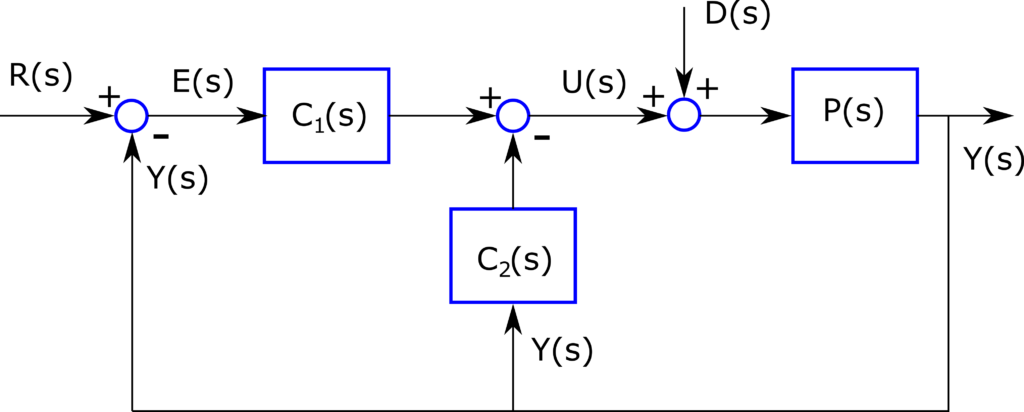
Structure of the two degrees of freedom controllers.

We have two controllers $C_{1}(s)$ and $C_{2}(s)$ , and a plant $P(s)$ . Here, $s$ is the Laplace complex variable, and capital letters denote that signals and models are expressed in the Laplace domain. $R(s)$ is the reference signal we want to track, and $Y(s)$ is the output.
Roughly speaking, since we have two controllers, we have two degrees of freedom when designing controllers. The classical PID control loop is obtained by erasing the controller $C_{2}(s)$ . The classical PID control loop has only a single degree of freedom since we only have a single controller. It should be noted that this is one of the possible control structures of two degrees of freedom PID controllers. Other structures will be discussed in our future tutorials.

Here is the problem we want to address:

Control Design Problem: For the plant model given by

(1) $\begin{align*}P(s)=\frac{5}{s(s+1)}\end{align*}$

Design the controllers $C_{1}(s)$ and $C_{2}(s)$ such that

a) The overshoot of tracking step reference signal $R(s)$ is below 25 percent.
b) The steady-state error of tracking step, ramp, and quadratic (acceleration) reference signals is zero.
c) The settling time of the system is smaller than $1.2$ seconds
d) The designed controllers are able to completely reject the step disturbance signals $D(s)$ .

Solution by using the zero-placement approach:

STEP 1: Derive the output-disturbance and output-reference transfer signals. From the block diagram in Fig. 1., we have

(2) $\begin{align*}& Y(s) =P(s)\big(D(s)+U(s)\big)=P(s)\big(D(s)+C_{1}(s)E(s)-C_{2}(s)Y(s) \big) \\& Y(s) =P(s)\Big(D(s)+C_{1}(s)\big(R(s)-Y(s) \big)-C_{2}(s)Y(s) \Big) \\& \Big(1+P(s)\big( C_{1}(s)+C_{2}(s) \big) \Big)Y(s) = P(s)D(s)+P(s)C_{1}(s)R(s) \\& Y(s)=\frac{P(s)}{1+P(s)\big( C_{1}(s)+C_{2}(s) \big) }D(s)+\frac{P(s)C_{1}(s)}{1+P(s)\big( C_{1}(s)+C_{2}(s) \big) }R(s)\end{align*}$

Let us define $C(s)$ as follows

(3) $\begin{align*}C(s)=C_{1}(s)+C_{2}(s)\end{align*}$

By using the last definition, we can define the following transfer functions

(4) $\begin{align*}W_{YD}(s)& =\frac{P(s)}{1+P(s)C(s)} \\W_{YR}(s)& =\frac{P(s)C_{1}(s)}{1+P(s)C(s)}\end{align*}$

Consequently, we can write (2) as follows

(5) $\begin{align*}Y(s)& = \frac{P(s)}{1+P(s)C(s) }D(s)+\frac{P(s)C_{1}(s)}{1+P(s)C(s) }R(s) \\Y(s)& = W_{YD}(s)D(s)+W_{YR}(s)R(s) \end{align*}$

Here, it is important to emphasize that our goal is to select the controllers $C_{1}(s)$ and $C_{2}(s)$ . We defined the new controller $C(s)$ that is a sum of $C_{1}(s)$ and $C_{2}(s)$ . This is an intermediate controller that is used to derive the controllers $C_{1}(s)$ and $C_{2}(s)$ .

STEP 2: Select the intermediate controller structure $C(s)$ such that the step disturbance is rejected. Let us select the intermediate controller $C(s)$ as follows

(6) $\begin{align*}C(s)=\frac{K}{s}(s+a)(s+b)\end{align*}$

where $K$ , $a$ , and $b$ are the controller parameters that need to be selected. By multiplying the controller coefficients, we can see that this is actually a PID controller:

(7) $\begin{align*}C(s)=Ks+(a+b)K+\frac{Kab}{s}\end{align*}$

Let us for a moment assume that $R(s)$ is zero, and let us substitute this controller in (5):

(8) $\begin{align*}Y(s)& =\frac{\frac{5}{s(s+1)}}{1+\frac{5}{s(s+1)}\frac{K}{s}(s+a)(s+b) }D(s) \\Y(s) & =\frac{5s}{s^2(s+1)+5K(s+a)(s+b)}D(s) \end{align*}$

Let us assume that the coefficients $K$ , $a$ , and $c$ are selected such that the system is stable. Then, by assuming that the disturbance signal is a step signal in the time domain (or $1/s$ in the Laplace domain), and by applying the finite value theorem:

(9) $\begin{align*}y(t=\infty)=\lim_{s-> 0 } s\frac{5s}{s^2(s+1)+5K(s+a)(s+b)}\cdot \frac{1}{s}=0\end{align*}$

where we assumed that all the zeros of $s^2(s+1)+5K(s+a)(s+b)$ are in the left half of the complex plane (stable system).

Consequently, an integrator component (1/s) in the controller $C(s)$ will ensure that the step disturbance can be rejected successfully. This is because the term $1/s$ from the denominator is transferred to the numerator. In the next step, we will select the parameters of the PID controller.

STEP 3: Use the zero placement approach to design the output-reference signal transfer function and the controller $C(s)$ .

First, it is important to observe that the terms in the denominator of the output-disturbance transfer function $W_{YD}$ and output-reference signal transfer function $W_{YR}$ are identical. This means that the characteristic polynomials of these two transfer functions are identical. That is, they will share the same poles.

On the other hand, notice that in the numerator of the transfer function $W_{YR}$ we have $C_{1}$ . That is, by wisely selecting the structure and parameters of this controller we can ensure that the zeros of $W_{YR}$ are designed such that the steady-state errors of tracking ramp and quadratic reference time signals are zero. The zero placement approach can be used to design such zeros.

To explain the main idea od the zero placement approach, let us consider the following transfer function

(10) $\begin{align*}W(s)=\frac{w(s)}{s^{n+1}+a_{n}s^{n}+a_{n-1}s^{n-1}+\ldots+a_{1}s+a_{0}}\end{align*}$

Let us assume that this system is stable. Our goal is to design the polynomial in the numerator $w(s)$ such that the steady-state errors of tracking step, ramp, and quadratic functions are zero. Let us compute the steady-state error

(11) $\begin{align*}&E(s)=R(s)-Y(s)\\&=\Big(1-W(s) \Big)R(s) \\& =\Big(\frac{s^{n+1}+a_{n}s^{n}+a_{n-1}s^{n-1}+\ldots+a_{1}s+a_{0}-w(s)}{s^{n+1}+a_{n}s^{n}+a_{n-1}s^{n-1}+\ldots+a_{1}s+a_{0}} \Big)R(s)\end{align*}$

Let us select the polynomial $w(s)$ to be equal to the last three entries of the polynomial in the denominator:

(12) $\begin{align*}w(s)=a_{2}s^{2}+a_{1}s+a_{0}\end{align*}$

Then, the error becomes

(13) $\begin{align*}E(s)=\Big(\frac{s^{n+1}+a_{n}s^{n}+\ldots+a_{3}s^{3}}{s^{n+1}+a_{n}s^{n}+a_{n-1}s^{n-1}+\ldots+a_{1}s+a_{0}} \Big)R(s)\end{align*}$

Now, let us show that this approach will produce zero tracking errors for step, ramp, and quadratic reference signals in the time domain.

Step input: $r(t)=1$ and $R(s)=\frac{1}{s}$
(14) $\begin{align*}& e_{\text{step}}(\infty)= \\& = \lim_{s-> 0} s\cdot \Big(\frac{s^{n+1}+a_{n}s^{n}+\ldots+a_{3}s^{3}}{s^{n+1}+a_{n}s^{n}+a_{n-1}s^{n-1}+\ldots+a_{1}s+a_{0}} \Big)\cdot \frac{1}{s} \\& e_{\text{step}}(\infty)=0\end{align*}$
Ramp input $r(t)=t$ and $R(s)=\frac{1}{s^{2}}$

(15) $\begin{align*}& e_{\text{ramp}}(\infty) = \\& = \lim_{s-> 0} s\cdot \Big(\frac{s^{n+1}+a_{n}s^{n}+\ldots+a_{3}s^{3}}{s^{n+1}+a_{n}s^{n}+a_{n-1}s^{n-1}+\ldots+a_{1}s+a_{0}} \Big)\cdot \frac{1}{s^2} \\& e_{\text{ramp}}(\infty)=0\end{align*}$
Quadratic input (acceleration input) $r(t)=t^2$ and $R(s)=\frac{2}{s^{2}}$
(16) $\begin{align*}& e_{\text{acc}}(\infty)= \\& = \lim_{s-> 0} s\cdot \Big(\frac{s^{n+1}+a_{n}s^{n}+\ldots+a_{3}s^{3}}{s^{n+1}+a_{n}s^{n}+a_{n-1}s^{n-1}+\ldots+a_{1}s+a_{0}} \Big)\cdot \frac{2}{s^3} \\& e_{\text{acc}}(\infty)=0\end{align*}$

Let us now apply this approach to our problem. We will combine the zero placement approach with the pole placement approach. That is, we will parameterize the transfer function.

The denominator of the transfer function $W_{YR}$ is equal to the denominator of the transfer function $W_{YD}$ that is derived in (8) and that is equal to

(17) $\begin{align*}& s^{2}(s+1)+5K(s+a)(s+b)=\\& =s^{3}+(1+5K)s^{2}+5K(a+b)s+5Kab\end{align*}$

We can observe that the polynomial in the denominator of $W_{YR}$ is of a 3rd order. Our goal is to design the parameters $a$ , $b$ , and $K$ , such that the desired transient response specifications are met. We will use the pole placement method to find these parameters. Since the denominator polynomial is of the 3rd order, this means that we need to select three poles. Let these poles be parametrized by

(18) $\begin{align*}s_{1}=- \gamma, \\s_{2}=-\alpha+j\beta \\s_{3}=-\alpha-j\beta\end{align*}$

where $\alpha$ , $\beta$ , and $\gamma$ are positive numbers that parameterize the location of poles.

The desired characteristic polynomial has the following form

(19) $\begin{align*}q(s)=(s+\gamma)(s+\alpha -j\beta)(s+\alpha +j\beta)\end{align*}$

This polynomial can be expressed as follows

(20) $\begin{align*}& q(s)=(s+\gamma)(s+\alpha -j\beta)(s+\alpha +j\beta) \\& q(s)=(s+\gamma)((s+\alpha)^{2}-(j\beta)^2) \\& q(s)=(s+\gamma)((s+\alpha)^{2}+\beta^2) \\& q(s) =s^3+(2\alpha +\gamma)s^{2}+(\alpha^2+\beta^2+2\alpha\gamma)s+\gamma(\alpha^2+\beta^2)\end{align*}$

From the structure of the last polynomial, we conclude that the transfer function can be parametrized as follows

(21) $\begin{align*}W_{YR}=\frac{(2\alpha +\gamma)s^{2}+(\alpha^2+\beta^2+2\alpha\gamma)s+\gamma(\alpha^2+\beta^2)}{s^3+(2\alpha +\gamma)s^{2}+(\alpha^2+\beta^2+2\alpha\gamma)s+\gamma(\alpha^2+\beta^2)}\end{align*}$

where we used the zero placement method in order to ensure that the last three terms of the numerator are equal to the last three terms of the denominator.

We will use a simple grid search in MATLAB to search for the parameters $\alpha$ , $\beta$ , and $\gamma$ that meet the transient response specifications. To perform the grid search, we need to determine the regions of these parameters.

To find these regions, we need to recall the formulas that relate the maximal overshoot and sampling time with the damping ratio and natural undamped frequency. These formulas are

(22) $\begin{align*}M_{\text{max}}=e^{\frac{-\pi \zeta}{\sqrt{1-\zeta^2}}}\end{align*}$

(23) $\begin{align*}t_{s}\approx \frac{3.2}{\zeta \omega_{n}}\end{align*}$

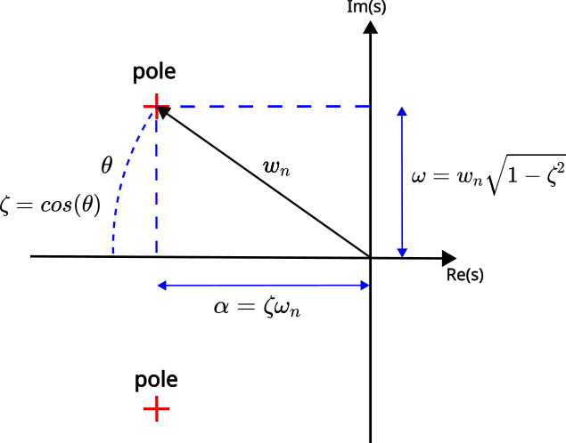
where $M_{\text{max}}$ is the maximum overshoot, $t_{s}$ is the settling time, $\zeta$ is the damping ratio, and $\omega_{n}$ is the natural undamped frequency. Here, it should be kept in mind that these formulas are derived under the assumption that the transfer function is a second-order prototype function. Despite the fact that we have a third order transfer function, these formulas can still be useful by ensuring that the third real pole parametrized by $\gamma$ is further away to the left in the complex plane from the two complex poles. When connecting the parameters $\zeta$ and $\omega_{n}$ with the poles, the graph presented below is useful

Figure 2: Illustration of the parameters $\zeta$ and $\omega_{n}$ .

From (22), we have

(24) $\begin{align*}\zeta=\sqrt{\frac{\ln^{2}(M_{\text{max}})}{\pi^{2}+\ln^{2}(M_{\text{max}})}}\end{align*}$

On the other hand, from (23), we have

(25) $\begin{align*}\omega_{n} \approx \frac{3.2}{\zeta t_{s}}\end{align*}$

The specification is that the overshoot is less than 25 percent. This corresponds to

(26) $\begin{align*}M_{\text{max}1}=0.25\end{align*}$

However, we need to specify a lower bound on the overshoot in order to avoid slow transient responses. We choose a minimum value of overshoot of $4$ percent. Consequently, we have

(27) $\begin{align*}M_{\text{max}2}=0.04\end{align*}$

Substituting these values in (24), we obtain the following values of $\zeta$

(28) $\begin{align*}\zeta_{1}=0.4037, \;\; \zeta_{2}=0.7156\end{align*}$

That is, the damping ratio that ensures the desired overshoot, should be in the interval

(29) $\begin{align*}0.4037\le \zeta \le 0.7156\end{align*}$

Consequently, by taking into account that $\zeta=\cos (\theta)$ , these two values correspond to the following angle $\theta$

(30) $\begin{align*}44.3039 \le \theta \le 66.1895\end{align*}$

On the other hand, for the computed bounds on $\zeta$ (bounds $\zeta_{1}$ and $\zeta_{2}$ ), and from the requirement on the settling time (below 1.2 second), and by using the formula (25), we obtain the following bounds on $\omega_{n}$ :

(31) $\begin{align*}3.7262 \le \omega_{n}\le 6.6054\end{align*}$

The equations (30) and (31) define a disc segment in the complex plane. By using this formula

(32) $\begin{align*}x=\omega_{n}\cos (\theta),\;\; y=\omega_{n}\sin (\theta)\end{align*}$

we can compute the coordinates of the segment edge points. The segment is shown in the figure below

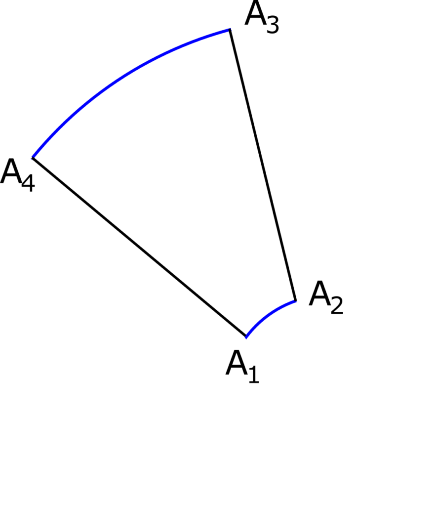
Figure 3: Segment in the complex plane corresponding to the pole locations.

The coordinates are

(33) $\begin{align*}A_{1}=(-2.6667,2.6026),\; A_{2}=(-1.5043,3.4091),\; \\ A_{3}=(-2.6667,6.0431),\; A_{4}=(-4.7271,4.6136)\end{align*}$

The MATLAB code for computing the bounds on $\zeta$ and $\omega_{n}$ , and for computing the coordinates is given below

clear

ub=0.25
lb=0.04


s1=log(ub)
s2=log(lb)

zeta1=sqrt((s1^2)/(pi^2+s1^2))
zeta2=sqrt((s2^2)/(pi^2+s2^2))

theta_upper=acosd(zeta1)
theta_lower=acosd(zeta2)


ts=1.2
wupper=3.2/(zeta1*ts)
wlower=3.2/(zeta2*ts)

% wn2<=omega<=wn1
% zeta1<=zeta<=zeta2

pointA1x=wlower*cosd(theta_lower)
pointA1y=wlower*sind(theta_lower)

pointA2x=wlower*cosd(theta_upper)
pointA2y=wlower*sind(theta_upper)


pointA3x=wupper*cosd(theta_upper)
pointA3y=wupper*sind(theta_upper)

pointA4x=wupper*cosd(theta_lower)
pointA4y=wupper*sind(theta_lower)

This segment can help us to select the search region for the parameters $\alpha$ and $\beta$ . For computational purposes, we select rectangular search regions. These search regions should contain the segment. We should keep in mind that we parametrized the controller such that $\alpha$ , $\beta$ , and $\gamma$ are positive. We select the following search region for $\alpha$ :

(34) $\begin{align*}1.4 \le \alpha \le 5\end{align*}$

We select the following search region for $\beta$

(35) $\begin{align*}2.5 \le \beta \le 6.2\end{align*}$

The search region for the $\gamma$ is

(36) $\begin{align*}6.2 \le \gamma \le 12\end{align*}$

We selected the search region for gamma such that the pole corresponding to $\gamma$ is further left in the complex plane compared to the poles parametrized by $\alpha$ and $\beta$ .

Next, our goal is to perform a grid search in order to determine the optimal values of the parameters $\alpha$ , $\beta$ , and $\gamma$ that will guarantee that the transient response of the parametrized transfer function (21) meets the design specifications. We vary the parameters $\alpha$ , $\beta$ , and $\gamma$ , and for every selection of these parameters we compute a transient response. If the transient response meets the specifications, we memorize the parameters $\alpha$ , $\beta$ , and $\gamma$ . In this way, we obtain a set of parameters that produce the desired response. The MATLAB code is given below.

clear,clc

% bounds
alpha_lower=1.4;
alpha_upper=5;

beta_lower=2.5;
beta_upper=6.2;

gamma_lower=6.2;
gamma_upper=12;


alpha=alpha_lower:0.1:alpha_upper;
beta=beta_lower:0.1:beta_upper;
gamma=gamma_lower:0.1:gamma_upper;

% bounds on the overshoot
overShootUpper=0.25;
overShootLower=0.04;

% simulation time
timeInput=0:0.01:10;

% coefficients
coefficientSelection=[];

for index_a=1:numel(alpha)
    % here track the progress
    (index_a/numel(alpha))*100
    for index_b=1:numel(beta)
        for index_c=1:numel(gamma)
            num=[(2*alpha(index_a)+gamma(index_c)), (alpha(index_a)^2+beta(index_b)^2+2*alpha(index_a)*gamma(index_c)), (alpha(index_a)^2+beta(index_b)^2)*gamma(index_c)];
            den=[1,(2*alpha(index_a)+gamma(index_c)), (alpha(index_a)^2+beta(index_b)^2+2*alpha(index_a)*gamma(index_c)), (alpha(index_a)^2+beta(index_b)^2)*gamma(index_c)];
            W=tf(num,den);
            [output,timeReturned]=step(W,timeInput);
            maxOutput=max(output);
            overShoot=maxOutput-1;
                 
            errorStep=output-ones(size(output));
                if (overShoot<overShootUpper) & (overShoot>overShootLower)
                    i=length(errorStep);
                    while (abs(errorStep(i))<0.02)
                        i=i-1;
                    end
                    
                    if (timeInput(i)<1)
                        coefficientSelection=[coefficientSelection;
                                              index_a,index_b,index_c,alpha(index_a),beta(index_b),gamma(index_c),timeInput(i),overShoot];
                    end
                end
        end
    end
end

% Select one model
index_a=37; index_b=21; index_c=50;
% this corresponds to
% alpha=5, beta=4.5, gamma=11.1

 num=[(2*alpha(index_a)+gamma(index_c)), (alpha(index_a)^2+beta(index_b)^2+2*alpha(index_a)*gamma(index_c)), (alpha(index_a)^2+beta(index_b)^2)*gamma(index_c)];
            den=[1,(2*alpha(index_a)+gamma(index_c)), (alpha(index_a)^2+beta(index_b)^2+2*alpha(index_a)*gamma(index_c)), (alpha(index_a)^2+beta(index_b)^2)*gamma(index_c)];
 W=tf(num,den);
 step(W)

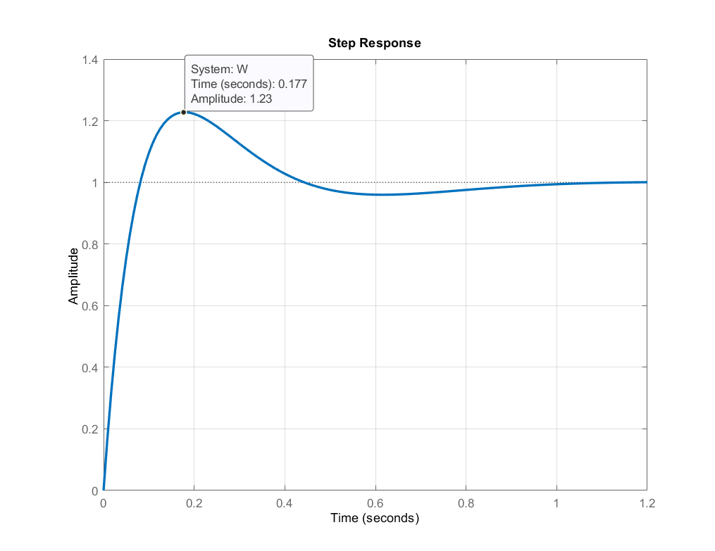
We select the following model:

(37) $\begin{align*}\alpha=5, \;\; \beta=4.5, \;\; \gamma=11.1\end{align*}$

These parameters produce the step response shown below.

Figure 4: Step response of the output-reference signal transfer function.

On the basis of the computed parameter values, we can determine the coefficients of the controller $C(s)$ . From (17), we can see that the parametrized characteristic polynomial is

(38) $\begin{align*}s^{3}+(1+5K)s^{2}+5K(a+b)s+5Kab\end{align*}$

and this characteristic polynomial should match the characteristic polynomial (20), that is repeated here for clarity:

(39) $\begin{align*}q(s) =s^3+(2\alpha +\gamma)s^{2}+(\alpha^2+\beta^2+2\alpha\gamma)s+\gamma(\alpha^2+\beta^2)\end{align*}$

By substituting the computed values of $\alpha$ , $\beta$ , and $\gamma$ in the last equation, we obtain

(40) $\begin{align*}q(s) =s^3+21.1s^{2}+156.25s+502.2750\end{align*}$

By equating (38) and (40), we obtain

(41) $\begin{align*}(1+5K)=21.1 \\5K(a+b)=156.25 \\5Kab=502.2750\end{align*}$

This is a system of 3 equations with three unknowns. From the first equation, we obtain

(42) $\begin{align*}K=\frac{21.1-1}{5}=4.02\end{align*}$

By substituting this computed value of $K$ in equations 2 and 3, and after some manipulation, we obtain

(43) $\begin{align*}a+b=7.7736 \\ab=24.9888\end{align*}$

We actually do not need to solve this system of equations, since the controller $C(s)$ is determined by

(44) $\begin{align*}C(s)=\frac{K}{s}(s+a)(s+b)=\frac{K}{s}(s^2+(s+b)s+ab)\end{align*}$

That is, the sum and product of $a$ and $b$ determine the controller $C$ . The controller $C(s)$ is given by

(45) $\begin{align*}C(s)=\frac{K}{s}(s^2+7.7736 s+24.9888)\end{align*}$

STEP 4: Design the controllers $C_{1}(s)$ and $C_{2}(s)$

We design the controller $C_{1}(s)$

admin

You might also like

The Correct Definition of the Fluid Flow Rate and Average Fluid Flow Rate – Derivation of the Formula Q=V*A

Correct and Intuitive Explanation of Observability of Linear Dynamical Systems

Some questions for the midterm exam