Free Fall of an Object (Ball) With Aerodynamic Drag Force – Fusion of Engineering, Control, Coding, Machine Learning, and Science

In this physics and dynamics tutorial, we explain how to solve the problem of the free fall of an object (ball) under the influence of an aerodynamic drag force. We analytically solve a differential equation describing the dynamics of a free-fall object and we analytically compute the expression for the velocity. The YouTube video accompanying this post is given below.

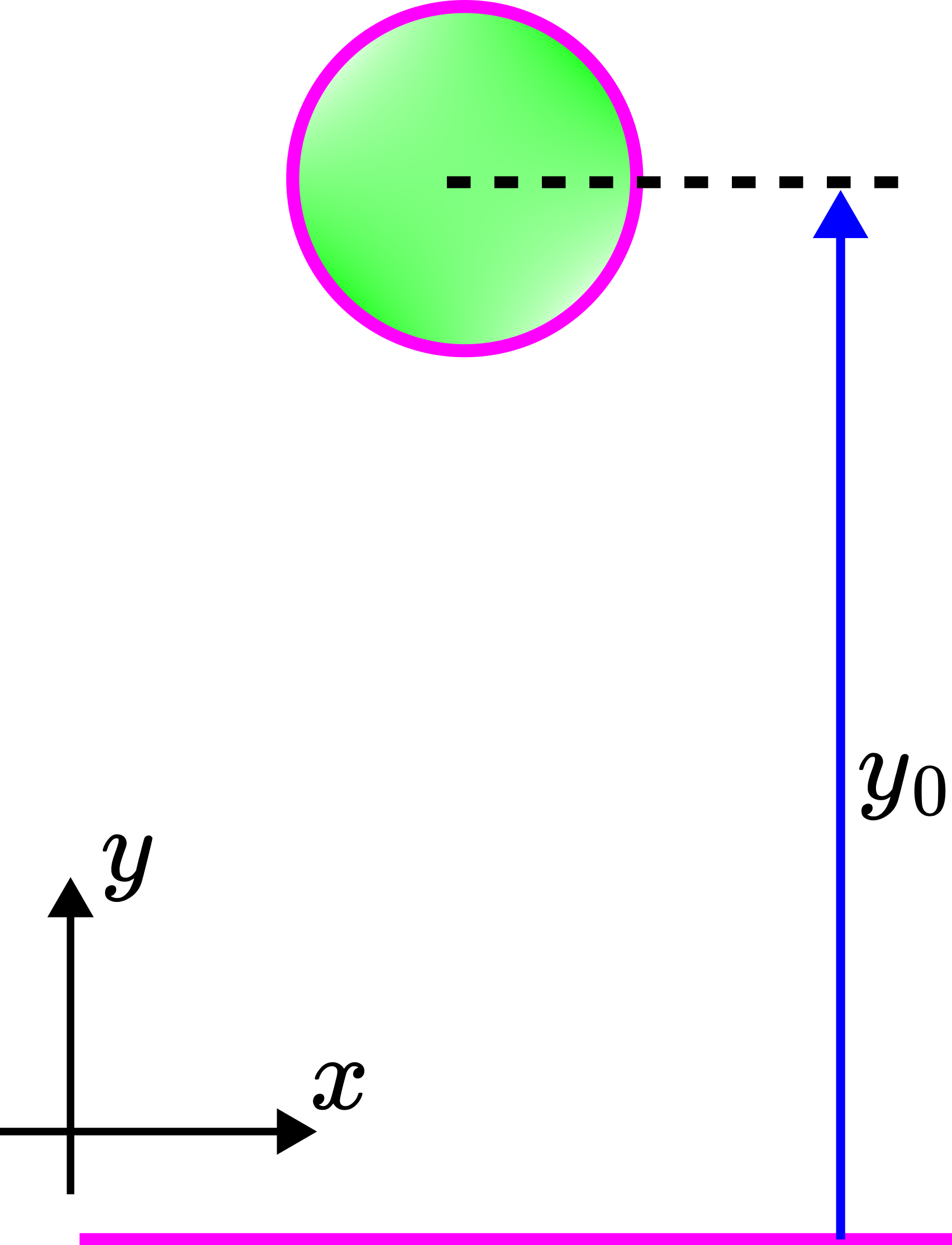
Problem: A ball with a mass of $m$ freely falls from the initial height of $y_{0}$ . The initial velocity of the ball is $0$ . The intensity of the aerodynamic drag force acting on the ball is $F_{D}=k\cdot v^{2}$ , where $k$ is a constant, and $v$ is the current velocity of the ball at the time instant $t$ . We assume that the buoyancy force can be neglected. Determine:

The velocity of the ball before it reaches the ground.
The velocity of the ball at the moment it hits the ground.
The steady-state velocity of the ball (assume that the steady-state velocity is reached before the ball reaches the ground).

Solution: The first step is to construct a free-body diagram. The free-body diagram is given below

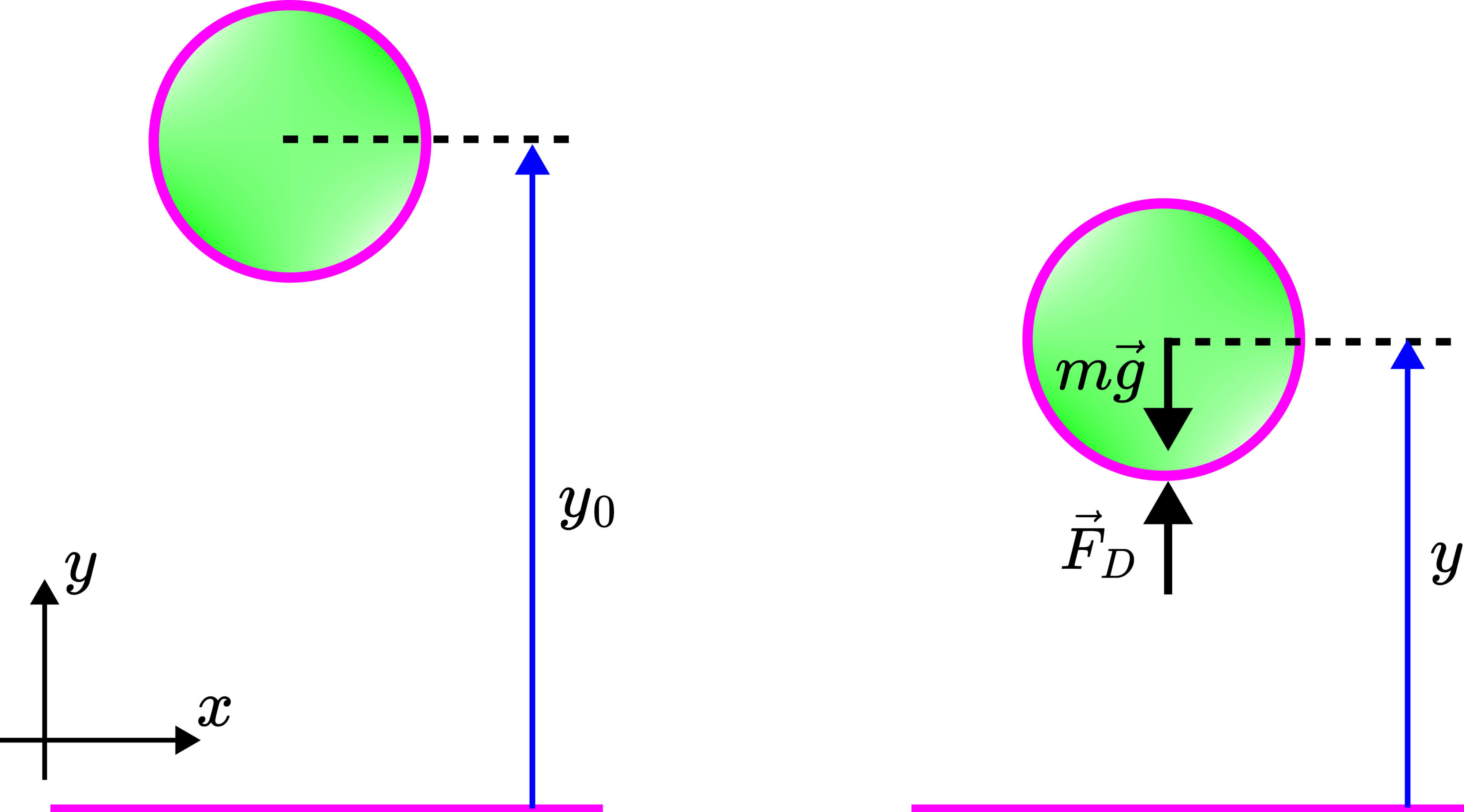
The gravity force $m\vec{g}$ and the aerodynamic drag force $\vec{F}_{D}$ act on the ball.

From Newton’s second law, we obtain

(1) $\begin{align*}m \vec{a}=m\vec{g}+\vec{F}_{D}\end{align*}$

where $a$ is the acceleration of the ball. Note here that we model the dynamics of the ball by assuming that the ball is a material point. By projecting this equation onto the $y$ axis, we obtain

(2) $\begin{align*}ma=-mg+kv^{2}\end{align*}$

where $a$ is the projection of the acceleration on the $y$ axis and $g$ is the gravitational acceleration constant. By using the fact that

(3) $\begin{align*}a=\frac{\text{d}v}{\text{d}t}\end{align*}$

We can write the last equation as follows

(4) $\begin{align*}m\frac{\text{d}v}{\text{d}t}=-mg+kv^{2}\end{align*}$

Next, we can write the last equation as follows

(5) $\begin{align*}m\frac{\text{d}y}{\text{d}t}\frac{\text{d}v}{\text{d}y}=-mg+kv^{2}\end{align*}$

By using the fact that

(6) $\begin{align*}v=\frac{\text{d}y}{\text{d}t}\end{align*}$

and by substituting this expression in (5), we have

(7) $\begin{align*}mv\frac{\text{d}v}{\text{d}y}=-mg+kv^{2}\end{align*}$

The last equation can be written as follows

(8) $\begin{align*}\frac{mv\text{d}v}{-mg+kv^{2}}=\text{d}y\end{align*}$

The last integral can be solved by using a substitution. The result is a $\ln (\cdot)$ function. Since the argument of this function has to be positive, we write the last equation as follows

(9) $\begin{align*}-\frac{mv\text{d}v}{mg-kv^{2}}=\text{d}y\end{align*}$

By using the substitution, we have

(10) $\begin{align*}s=mg-kv^{2} \\\text{d}s=-2kv\text{d}v \\v\text{d}v=-\frac{\text{d}s}{2k}\end{align*}$

By substituting (10) in the left side of (9), we obtain

(11) $\begin{align*}\frac{1}{2k}\frac{m\text{d}s}{s}\end{align*}$

By integrating this expression, we have

(12) $\begin{align*}\frac{m}{2k}\ln (s)\end{align*}$

By substituting the first equation of (10) in (12) we obtain:

(13) $\begin{align*}-\int \frac{mv\text{d}v}{mg-kv^{2}} = \frac{m}{2k}\ln (mg-kv^{2})\end{align*}$

By integrating the left and right-hand side of and by using (13), we obtain

(14) $\begin{align*}\frac{m}{2k}\ln (mg-kv^{2})\bigg\rvert_{0}^{v_{c}}=y\bigg\rvert_{y_{0}}^{y_{c}} \\\frac{m}{2k} \left( \ln (mg-kv^{2}_{c})-\ln (mg) \right) =y_{c}-y_{0} \\\frac{m}{2k} \ln (\frac{mg-kv^{2}_{c}}{mg})=y_{c}-y_{0} \end{align*}$

where $y_{c}$ is the current height of the ball, and $v_{c}$ is the current velocity of the ball. From the last equation, we obtain

(15) $\begin{align*}\ln (\frac{mg-kv^{2}_{c}}{mg})=\frac{2k}{m} \big( y_{c}-y_{0} \big) \\\frac{mg-kv^{2}_{c}}{mg}=e^{\frac{2k}{m} \big( y_{c}-y_{0} \big)} \\1-\frac{kv^{2}_{c}}{mg}=e^{\frac{2k}{m} \big( y_{c}-y_{0} \big)} \\v^{2}_{c}=\frac{mg}{k}\big( 1-e^{\frac{2k}{m} \big( y_{c}-y_{0} \big)}\big)\end{align*}$

The final expression is

(16) $\begin{align*}v_{c}=\sqrt{\frac{mg}{k}\big( 1-e^{\frac{2k}{m} \big( y_{c}-y_{0} \big)}\big)}\end{align*}$

The velocity at the moment of hitting the ground is obtained for $y_{c}=0$

(17) $\begin{align*}v_{c}=\sqrt{\frac{mg}{k}\big( 1-e^{\frac{2k}{m} \big(-y_{0} \big)}\big)}\end{align*}$

The steady-state velocity (terminal velocity) is obtained from (2), for $a=0$ . This means that the velocity is constant. From (2), we obtain

(18) $\begin{align*}0=-mg+kv^{2}_{ss}\end{align*}$

where $v_{ss}$ is the steady-state velocity. From (18), we obtain

(19) $\begin{align*}v_{ss}=\sqrt{\frac{mg}{k}}\end{align*}$

admin

You might also like

Fanuc Robot Tutorial 1: Starting the Robot, Clearing Faults, and Jogging Modes (Joint and World)

Introduction to Kalman Filter: Disciplined Python Implementation of Recursive Least Squares Method

Inverse Laplace Transform by Using Partial Fraction Expansion and Cover-Up Method – Case of (Real) Distinct Poles