Easy-to-Understand Explanation of Controllable Canonical Form – (also known as Reachable or Control Canonical form) – Fusion of Engineering, Control, Coding, Machine Learning, and Science

In this control theory and control engineering tutorial, we provide an easy-to-understand explanation of the controllable canonical form. The controllable canonical form is also known as the reachable canonical form or control canonical form. The YouTube video accompanying this tutorial is given below.

Motivation for Studying Controllable Canonical Form

Generally speaking, the controllable canonical form is a state-space description of the system in which all the system modes are controllable. Namely, it can be shown that the determinant of the controllability matrix of the state-space model in the controllable canonical form is equal to one, and consequently, the system is controllable.

The controllable canonical form serves as the basis of a number of control and estimation methods. For us, the most important method is the pole placement method. Namely, by creating the controllable canonical state-space description, we can easily determine the characteristic polynomial of the system, and we can easily assign the poles of the closed-loop system by using the state feedback. This is explained in the tutorial on pole placement by using the controllable canonical form that is given over here.

The Main Idea of the Controllable Canonical Form

We explain the main idea of the controllable canonical form by considering a third-order system. However, everything explained in the sequel can easily be generalized to systems of arbitrary order. The main idea of the controllable canonical form is explained by using the following example:

(1) $\begin{align*}\frac{Y(s)}{U(s)}=W(s)=\frac{b_{1}s^{2}+b_{2}s+b_{3}}{s^{3}+a_{1}s^{2}+a_{2}s+a_{3}}\end{align*}$

This is a third-order transfer function, $Y(s)$ is the output of the system in the Laplace domain $s$ , $U(s)$ is the input of the system in the Laplace domain, and $W(s)$ is the transfer function. Our goal is to write down a state-space model of the system (1). For that purpose, we write the original system in this form

(2) $\begin{align*}& \frac{Y(s)}{U(s)}=\frac{Y(s)}{P(s)}\frac{P(s)}{U(s)}=W_{PY}(s)\cdot W_{UP}(s) \\& \frac{Y(s)}{P(s)}=W_{PY}=b_{1}s^{2}+b_{2}s+b_{3},\\ & \frac{P(s)}{U(s)}=W_{UP}=\frac{1}{s^{3}+a_{1}s^{2}+a_{2}s+a_{3}}\end{align*}$

where $P(s)$ is the Laplace transform of the variable $p(t)$ ( $p(t)$ is in the time domain). The variable $p(t)$ is usually called the partial state.

First, we focus on the transfer function $W_{UP}$ :

(3) $\begin{align*}\frac{P(s)}{U(s)}=W_{UP}=\frac{1}{s^{3}+a_{1}s^{2}+a_{2}s+a_{3}}\end{align*}$

From this transfer function, we have

(4) $\begin{align*}\Big( s^{3}+a_{1}s^{2}+a_{2}s+a_{3}\Big) P(s)=U(s)\end{align*}$

or in the time domain

(5) $\begin{align*}p^{(3)}+a_{1}\ddot{p}+a_{2}\dot{p}+a_{3}p=u \end{align*}$

where $p^{(3)}$ is the third derivative of $p(t)$ , $\ddot{p}$ is the second derivative, and $\dot{p}$ is the first derivative. We obtained this time-domain description of the system by keeping in mind that $s^{v}P(s)$ in the complex $s$ domain is equivalent to $p^{(v)}(t)$ in the time domain, where $v$ is an arbitrary positive integer and $p^{(v)}(t)$ is the $v$ -th derivative of $p(t)$ . The equation (5), can be written as follows

(6) $\begin{align*}p^{(3)}=-a_{1}\ddot{p}-a_{2}\dot{p}-a_{3}p+u \end{align*}$

On the other hand, consider the function $W_{PY}$ :

(7) $\begin{align*}\frac{Y(s)}{P(s)}=W_{PY}=b_{1}s^{2}+b_{2}s+b_{3}\end{align*}$

In the time domain, this system has the following form

(8) $\begin{align*}y=b_{1}\ddot{p}+b_{2}\dot{p}+b_{3}p\end{align*}$

The equations (6) and (8) enable us to write a state-space model in the controllable canonical form. From (6), we can see that the following state variable assignment

(9) $\begin{align*}x_{1}=\ddot{p},\;\; x_{2}=\dot{p},\;\; x_{3}=p\end{align*}$

will produce the following equation

(10) $\begin{align*}\dot{x}_{1}=-a_{1}x_{1}-a_{2}x_{2}-a_{3}x_{3}+u \end{align*}$

On the other hand, from (8) and by using (9), we obtain the following output equation

(11) $\begin{align*}y=b_{1}x_{1}+b_{2}x_{2}+b_{3}x_{3}\end{align*}$

By using (9), (10), and (11), we obtain the following state-space model

(12) $\begin{align*}\begin{bmatrix}\dot{x}_{1} \\ \dot{x}_{2} \\ \dot{x}_{3}\end{bmatrix} & = \begin{bmatrix}-a_{1} & -a_{2} & -a_{3} \\ 1 & 0 & 0 \\ 0 & 1 & 0 \end{bmatrix}\begin{bmatrix} x_{1}\\ x_{2}\\ x_{3} \end{bmatrix}+\begin{bmatrix} 1 \\ 0 \\ 0 \end{bmatrix} u \\y & =\begin{bmatrix}b_{1} & b_{2} & b_{3} \end{bmatrix}\begin{bmatrix} x_{1} \\ x_{2} \\ x_{3} \end{bmatrix}\end{align*}$

The last equation can be written compactly

(13) $\begin{align*}\dot{\mathbf{x}} & =A\matbf{x}+B\mathbf{u} \\\mathbf{y}& =C\mathbf{x}\end{align*}$

where

(14) $\begin{align*}A=\begin{bmatrix} -a_{1} & -a_{2} & -a_{3} \\ 1 & 0 & 0 \\ 0 & 1 & 0 \end{bmatrix},\;\; B=\begin{bmatrix} 1 \\ 0 \\ 0 \end{bmatrix},\;\; \mathbf{x}=\begin{bmatrix}x_{1}\\ x_{2} \\ x_{3} \end{bmatrix} \\C=\begin{bmatrix} b_{1} & b_{2} & b_{3} \end{bmatrix}\end{align*}$

The equation (12) is the controllable canonical form. This form is also called the upper companion form.

The state-space model in the controllable canonical form is controllable

Here we will show that the state-space model in the controllable canonical form is controllable.

The controllability matrix is defined as

(15) $\begin{align*}\mathcal{C}=\begin{bmatrix} B & AB & A^{2}B \end{bmatrix}\end{align*}$

The system is controllable if and only if

(16) $\begin{align*}\text{rank}\Big(\mathcal{C} \Big) =3\end{align*}$

From (12), we see that

(17) $\begin{align*}B=\begin{bmatrix} 1 \\ 0 \\ 0 \end{bmatrix},\; AB=\begin{bmatrix} -a_{1} & -a_{2} & -a_{3} \\ 1 & 0 & 0 \\ 0 & 1 & 0 \end{bmatrix} \begin{bmatrix} 1 \\ 0 \\ 0 \end{bmatrix}=\begin{bmatrix} -a_{1} \\ 1\\0 \end{bmatrix} \\A^{2}B=A\cdot AB= \begin{bmatrix} -a_{1} & -a_{2} & -a_{3} \\ 1 & 0 & 0 \\ 0 & 1 & 0 \end{bmatrix}\begin{bmatrix} -a_{1} \\ 1\\0 \end{bmatrix} =\begin{bmatrix} a_{1}^{2}-a_{2}\\-a_{1}\\ 1 \end{bmatrix}\end{align*}$

Substituting (17) in (15), we obtain

(18) $\begin{align*}\mathcal{C}=\begin{bmatrix} 1 & -a_{1} & a_{1}^{2}-a_{2} \\ 0 & 1 & -a_{1} \\ 0 & 0 & 1 \end{bmatrix}\end{align*}$

The controllability matrix $\mathcal{C}$ is an upper triangular matrix. It can easily be shown that the determinant of the upper triangular matrix is equal to $1$ . Consequently, the system is controllable.

Creating a Block Diagram of the Controllable Canonical Form

Here, we explain how to create a block diagram of the controllable canonical form.

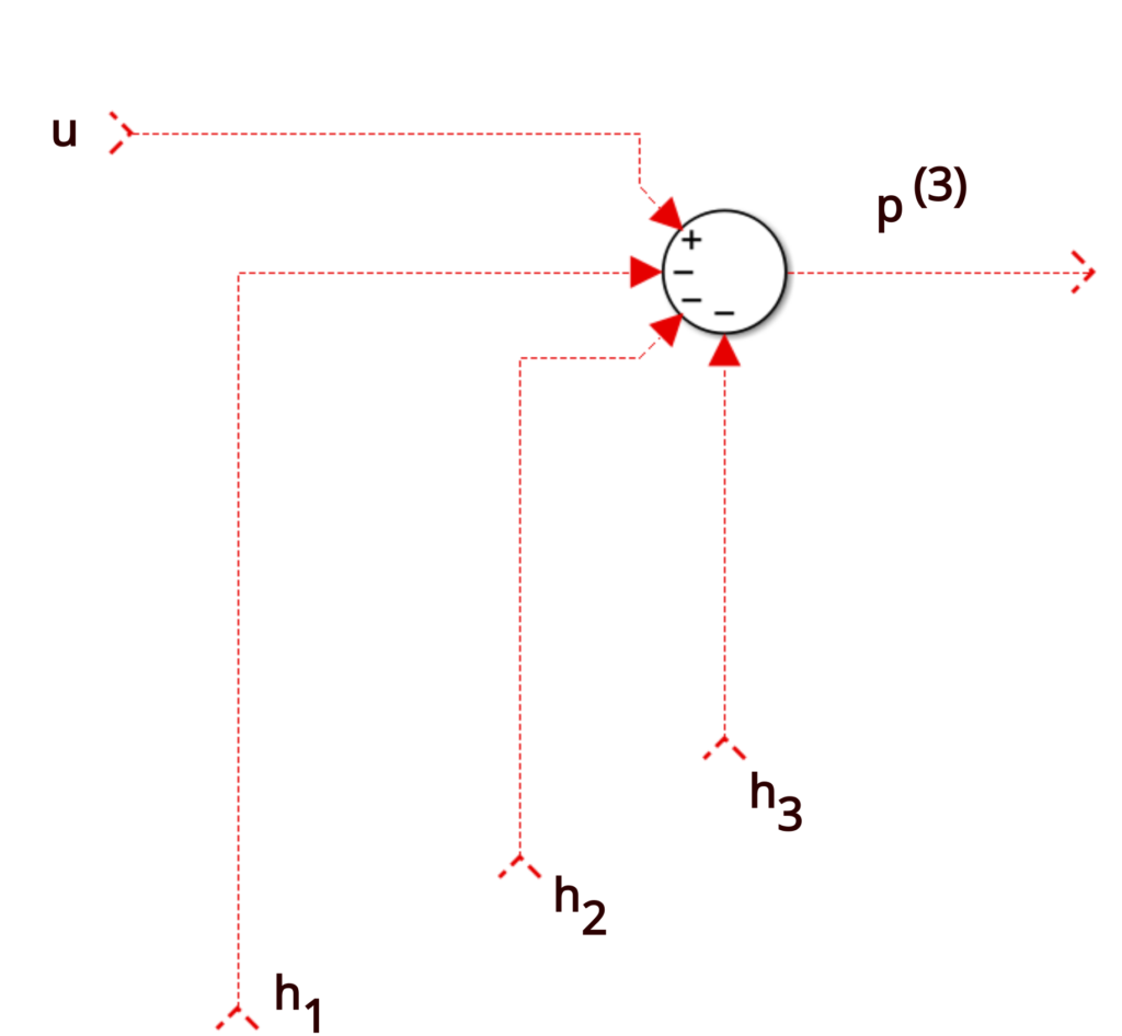
Let us focus on the equation (6). Here, we will rewrite this equation for ease of following this tutorial.

(19) $\begin{align*}p^{(3)}=- \underbrace{a_{1}\ddot{p}}_{h_{3}}-\underbrace{a_{2}\dot{p}}_{h_{2}}-\underbrace{a_{3}p}_{h_{1}}+u \end{align*}$

This is basically a summation block which is shown in the figure below.

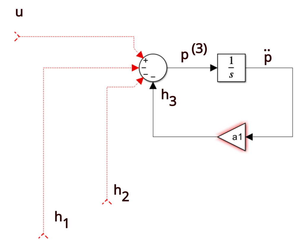
Figure 1: Summation block corresponding to the equation (19).

Next, we need to add the $h_{3}$ signal. We can do that by observing that $h_{3}$ signal is the feedback from $a_{1}\ddot{p}$ . Consequently, we need to add an integrator to produce $\ddot{p}$ from $p^{(3)}$ , and to add feedback with the gain of $a_{1}$ . This is shown in the figure below.

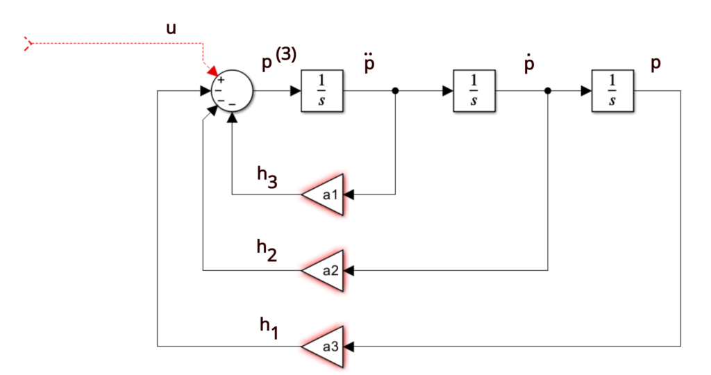
Figure 2: First integrator and feedback added.

By using the same procedure we add two integrators and two additional feedbacks corresponding to $h_{1}$ and h_{2}. Consequently, we obtain the diagram shown in the figure below.

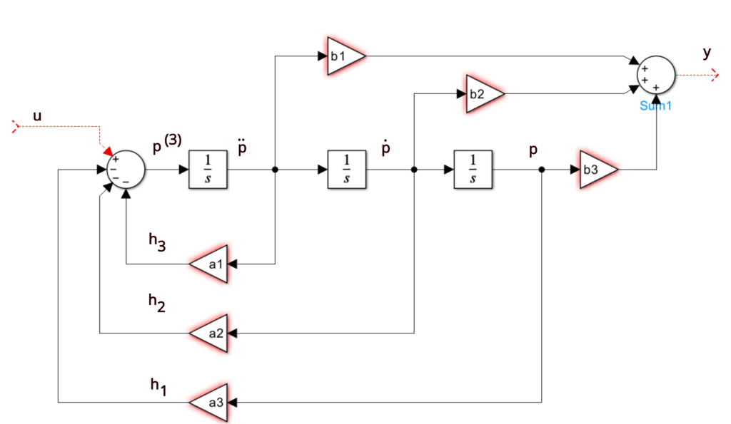
Figure 3: Block diagram corresponding to the equation (19).

Next, we need to add a part of the block diagram corresponding to the output equation (8). This equation is repeated here for completeness:

(20) $\begin{align*}y=b_{1}\ddot{p}+b_{2}\dot{p}+b_{3}p\end{align*}$

By using the same principle, we can add blocks corresponding to the output equation. As the result, we obtain the final block diagram shown in the figure below.

Motivation for Studying Controllable Canonical Form

The Main Idea of the Controllable Canonical Form

The state-space model in the controllable canonical form is controllable

Creating a Block Diagram of the Controllable Canonical Form

admin

You might also like

Gentle Introduction to Gradients and Level Curves (Surfaces)

Solve Constrained Optimization Problems in Python by Using SciPy Library, minimize() Function and Trust-Region Constrained Method

Direction Cosine Matrix Tutorial – Correct Mathematical Explanation -Important for Aerospace and Robotics Engineering