Solve Constrained Optimization Problems in Python by Using SciPy Library, minimize() Function and Trust-Region Constrained Method – Fusion of Engineering, Control, Coding, Machine Learning, and Science

In our previous post and tutorial which can be found here, we explained how to solve unconstrained optimization problems in Python by using the SciPy library and the minimize() function. In this post, we explain how to solve constrained optimization problems by using a similar approach.

The YouTube video accompanying this post is given below.

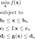
We use the trust-region constrained method to solve constrained minimization problems. This method assumes that the problems have the following form:

(1) $\begin{align*}& \min_{\mathbf{x}} f(\mathbf{x}) \\& \text{subject to} \\& \mathbf{b}_{l} \le \mathbf{x} \le \mathbf{b}_{u}\\& \mathbf{c}_{l} \le L \mathbf{x} \le \mathbf{c}_{u}\\& \mathbf{d}_{l} \le \mathbf{g}(\mathbf{x}) \le \mathbf{d}_{u}\end{align*}$

where

$\mathbf{x} \in \mathbb{R}^{n}$ is the n-dimensional vector of optimization variables
$f(\mathbf{x}):\mathbb{R}^{n}\rightarrow \mathbb{R}$ is the cost function
$\mathbf{b}_{l}, \mathbf{b}_{u}\in \mathbb{R}^{n}$ are the vectors of lower and upper bounds on the optimization variable $\mathbf{x}$
$\mathbf{c}_{l}, \mathbf{c}_{u}\in \mathbb{R}^{l}$ are the vectors of lower and upper bounds on the linear term $L \mathbf{x}$ , where $L\in \mathbb{R}^{l \times n}$ is a constant matrix of parameters. The compact notation
(2) $\begin{align*}\mathbf{c}_{l} \le L \mathbf{x} \le \mathbf{c}_{u}\end{align*}$

represents a set of $l$ linear “less than or equal to” constraints.
$\mathbf{d}_{l},\mathbf{d}_{u}\in \mathbb{R}^{p}$ are the vectors of lower and upper bounds on the nonlinear vector function $\mathbf{g}(\mathbf{x}): \mathbb{R}^{n} \rightarrow \mathbb{R}^{p}$ . The compact notation
(3) $\begin{align*}\mathbf{d}_{l} \le \mathbf{g}(\mathbf{x}) \le \mathbf{d}_{u}\end{align*}$

represents a set of “p” nonlinear “less than or equal to” constraints.

Here are a few comments about the above-presented generic problem. All the less-than or equal to inequalities are interpreted element-wise. For example, the notation

(4) $\begin{align*}\mathbf{b}_{l} \le \mathbf{x} \le \mathbf{b}_{u}\end{align*}$

is actually a shorthand notation for

(5) $\begin{align*}b_{l1}\le x_{1} \le b_{u1} \\b_{l2}\le x_{2} \le b_{u2} \\\mathbf{b}_{l}=\begin{bmatrix} b_{l1}\\ b_{l2} \end{bmatrix},\;\; \mathbf{b}_{u}=\begin{bmatrix} b_{u1}\\ b_{u2} \end{bmatrix},\;\; \mathbf{x}=\begin{bmatrix}x_{1} \\ x_{2} \end{bmatrix}\end{align*}$

where for simplicity, we assumed $n=2$ .

Then, the one-sided less than or equal to inequalities of the following form

(6) $\begin{align*}\mathbf{x}\le \mathbf{b}_{u}\end{align*}$

are formally written as follows

(7) $\begin{align*}& \mathbf{b}_{l} \le \mathbf{x}\le \mathbf{b}_{u} \\& \mathbf{b}_{l}=\begin{bmatrix} -\infty \\ -\infty \\ \vdots \\ -\infty \end{bmatrix}\end{align*}$

In a similar manner, we can formally write other types of one-sided less than or equal inequalities.

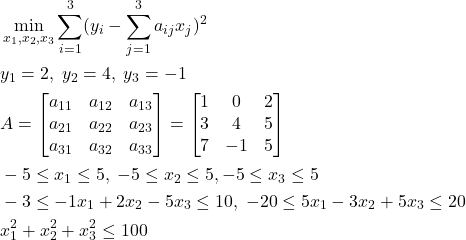
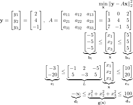
In order to illustrate how to transform particular problems in the above general form, we consider the following optimization problem:

(8) $\begin{align*}& \min_{x_{1},x_{2},x_{3}} \sum_{i=1}^{3} (y_{i}-\sum_{j=1}^{3}a_{ij}x_{j})^{2} \\& y_{1}=2,\;y_{2}=4, \; y_{3}=-1 \\& A=\begin{bmatrix}a_{11} & a_{12} & a_{13} \\ a_{21} & a_{22} & a_{23} \\ a_{31} & a_{32} & a_{33}\end{bmatrix}=\begin{bmatrix}1 & 0 & 2 \\ 3 & 4 & 5 \\ 7 & -1 & 5 \end{bmatrix} \\& -5\le x_{1} \le 5, \; -5\le x_{2} \le 5, -5\le x_{3} \le 5 \\& -3 \le -1x_{1}+2x_{2}-5x_{3} \le 10,\; -20 \le 5x_{1}-3x_{2}+5x_{3} \le 20 \\& x_{1}^{2}+x_{2}^{2}+x_{3}^{2}\le 100\end{align*}$

This problem can be compactly written as follows

(9) $\begin{align*}\min_{\mathbf{x}} \left\|\mathbf{y}-A\mathbf{x} \right\|_{2}^{2} \\\mathbf{y}=\begin{bmatrix} y_{1} \\ y_{2} \\ y_{3} \end{bmatrix} =\begin{bmatrix} 2\\ 4 \\-1 \end{bmatrix},\;\; A=\begin{bmatrix}a_{11} & a_{12} & a_{13} \\ a_{21} & a_{22} & a_{23} \\ a_{31} & a_{32} & a_{33}\end{bmatrix}=\begin{bmatrix}1 & 0 & 2 \\ 3 & 4 & 5 \\ 7 & -1 & 5 \end{bmatrix} \\\underbrace{\begin{bmatrix} -5 \\ -5 \\ - 5 \end{bmatrix}}_{\mathbf{b}_{l}} \le \underbrace{\begin{bmatrix} x_{1} \\ x_{2} \\ x_{3}\end{bmatrix}}_{\mathbf{x}} \le \underbrace{\begin{bmatrix} 5 \\ 5 \\ 5 \end{bmatrix}}_{\mathbf{b}_{u}} \\\underbrace{\begin{bmatrix}-3 \\ -20 \end{bmatrix}}_{\mathbf{c}_{l}} \le \underbrace{\begin{bmatrix} -1 & 2 & - 5 \\ 5 & -3 & 5 \end{bmatrix}}_{L}\underbrace{\begin{bmatrix} x_{1} \\ x_{2} \\x_{3}\end{bmatrix}}_{\mathbf{x}} \le \underbrace{\begin{bmatrix} 10 \\ 20 \end{bmatrix}}_{\mathbf{c}_{u}} \\ \underbrace{-\infty}_{\mathbf{d}_{l}} \le \underbrace{x_{1}^{2}+x_{2}^{2}+x_{3}^{2}}_{\mathbf{g}(\mathbf{x})} \le \underbrace{100}_{\mathbf{d}_{u}}\end{align*}$

where $\left\| \cdot \right\|_{2}$ denotes the vector 2-norm. The cost function is actually a least-squares cost function.

Now that we know how to transform problems in the general form, we can proceed with Python implementation. First, we import the necessary libraries and functions

import numpy as np 
import scipy
from scipy.optimize import minimize
from scipy.optimize import Bounds
from scipy.optimize import LinearConstraint
from scipy.optimize import NonlinearConstraint

We use the SciPy Python library and the functions minimize(), Bounds(), LinearConstraint(), and NonlinearConstraint() that are used to define and solve the problem. These functions will be explained in the sequel. But before we explain these functions, we need to construct our problem. Here, for simplicity of the implementation, we will not use the same coefficients as the coefficients used in (9). However, the structure of the problem is the same. We construct the problem with random vector $\mathbf{y}$ and the matrix $A$ :

# define a random matrix A that is our data matrix
A=np.random.randn(3,3)

# select the right-hand side
Y=np.random.randn(3,1)

Next, we need to define the cost function. We define the cost function as the following Python function

# define the cost function
def costFunction(x,Amatrix, Yvector):
    error=Yvector-np.matmul(Amatrix,x)
    returnValue=np.linalg.norm(error,2)**2
    return returnValue

Basically, this cost function for the given value of the optimization variable “x” and the matrix A and the vector $\mathbf{y}$ , returns the value of the cost function.

Next, we define the bounds, linear and nonlinear constraints:

# define the bounds 
lowerBounds= -1*np.inf*np.ones(3)
upperBounds=10*np.ones(3)
boundData=Bounds(lowerBounds,upperBounds)

#define the linear constraints
lowerBoundLinearConstraints=-1*np.inf*np.ones(3)
upperBoundLinearConstraints=30*np.ones(3)
matrixLinearConstraints=np.random.randn(3,3)
linearConstraints = LinearConstraint(matrixLinearConstraints, lowerBoundLinearConstraints, upperBoundLinearConstraints)

#define the nonlinear constraints
lowerBoundNonLinearConstraints=0
upperBoundNonLinearConstraints=100
def nonlinearConstraintMiddle(x):
    return x[0]**2+x[1]**2+x[2]**2

nonlinearConstraints = NonlinearConstraint(nonlinearConstraintMiddle, lowerBoundNonLinearConstraints, upperBoundNonLinearConstraints )

The bounds on $\mathbf{x}$ are specified by the function Bound() on the code line 4. This function accepts two arguments: lower and upper bounds. The linear constraints are defined on the code line 10 by using the function LinearConstraint(). The first argument of this function is the matrix $L$ , and the second and third arguments are lower and upper bounds. The nonlinear constraints are defined on the code lines 12 to 18. The nonlinear function $\mathbf{g}(\mathbf{x})$ is defined on the code lines 15 to 16. The nonlinear constraints are specified by the function NonlinearConstraint() on the code line 18. The first argument is the name of the function defining the vector function $\mathbf{g}(\mathbf{x})$ , and the second and third arguments are lower and upper bounds.

Finally, we can specify an initial guess of the solution and solve the optimization problem

## solve the optimization problem

# select the initial guess of the solution
x0=np.random.randn(3)


# see all the options for the solver
scipy.optimize.show_options(solver='minimize',method='trust-constr')

result = minimize(costFunction, x0, method='trust-constr', 
               constraints=[linearConstraints, nonlinearConstraints],
               args=(A, np.reshape(Y,(3,))),options={'verbose': 1}, bounds=boundData)

# here is the solution
result.x

We need an initial guess of the solution since we are using an iterative optimization method. The initial guess is specified on the code line 4. In our case, we use the Trust Region Constrained algorithm, that is specified by ‘trust-constr’. We can see all the options for the solver by using the function scipy.optimize.show_options(). We can see what are the parameters that we can change or adjust in order to achieve a better accuracy or to increase the number of iterations or function evaluations. We solve the problem by using the functioin minimize() on the code line 10. The first argument is the name of the cost function. The second argument is the initial guess of the solution. The method is specified as the third argument. The constraint functions are specified as the list, and this is the fourth argument. The fifth argument contains parameters that are sent to the cost function. These parameters are the matrix $A$ and the vector $\mathbf{y}$ . The last argument is a dictionary containing all the solution options. The minimize function returns the structure “result”. The solution can be accessed by typing result.x.

admin

You might also like

Cart Pole Control Environment in OpenAI Gym (Gymnasium)- Introduction to OpenAI Gym

4. Simple moving averages of stock time-series in Pandas and Python

Test 5