Cart Pole Control Environment in OpenAI Gym (Gymnasium)- Introduction to OpenAI Gym – Fusion of Engineering, Control, Coding, Machine Learning, and Science

In this tutorial, we introduce the Cart Pole control environment in OpenAI Gym or in Gymnasium. This Python reinforcement learning environment is important since it is a classical control engineering environment that enables us to test reinforcement learning algorithms that can potentially be applied to mechanical systems, such as robots, autonomous driving vehicles, rockets, etc. The GitHub page with the codes presented in this tutorial is given here. The YouTube video accompanying this tutorial is given below.

Summary of the Cart Pole Control Environment

The Cart Pole control environment is shown below.

It consists of a cart that can move linearly, and a rotating bar or a pole attached to it via a bearing. Another name for this system is the inverted pendulum. Although this is not a topic of this tutorial, we made a video demonstrating the control of an inverted pendulum by using a Proportional Integral Derivative (PID) control algorithm. This video is given below the figure.

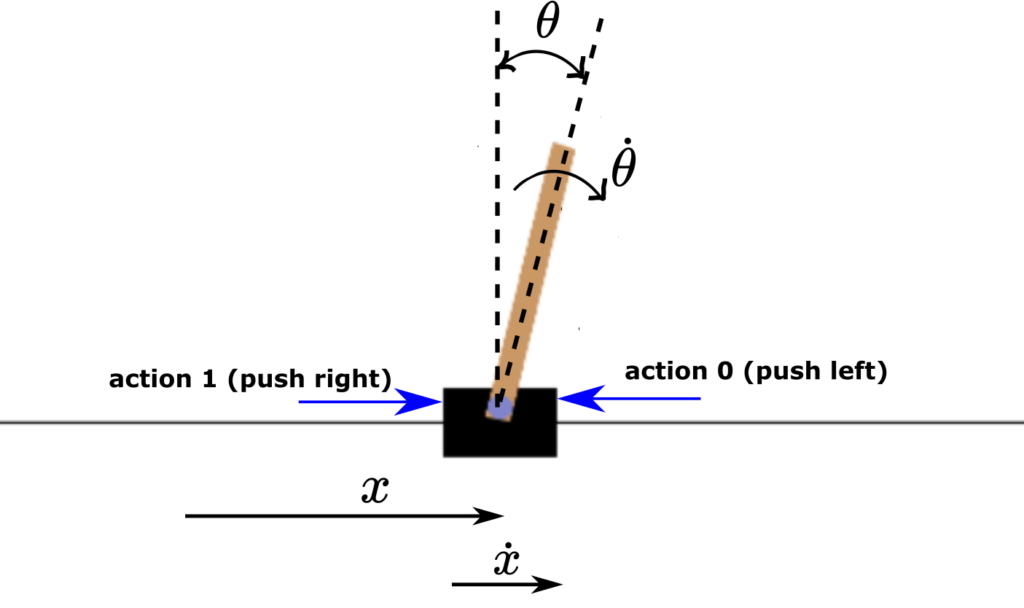
Figure 1: Cart Pole mechanical system in OpenAI Gym or Gymanisum environment.

The control objective is to keep the pole in the vertical position by applying horizontal actions (forces) to the cart. The action space consists of two actions

Push the cart left – denoted by 0
Push the cart right – denoted by 1

The observation space or the states are

Cart position, denoted by $x$ in Fig. 1. The minimal and maximal values are -4.8 and 4.8, respectively.
Cart velocity, denoted by $\dot{x}$ in Fig. 1. The minimal and maximal values are $-\infty$ and $\infty$ , respectively.
Pole angle of rotation (measured in radians), denoted by $\theta$ . The minimal and maximal values are -0.418 radians (-24 degrees) and 0.418 (24 degrees).
Pole angular velocity, denoted by $\dot{\theta}$ . The minimal and maximal values are $-\infty$ and $\infty$ , respectively.

Here it is also important to emphasize that initial states (initial observations) are completely random and the values of states are chosen uniformly from the interval (-0.05,0.05).

All observations are assigned a uniformly random value in (-0.05, 0.05)

An episode terminates under the following conditions:

Pole angle becomes greater than |12| degrees (absolute value of $\pm 12$ ) or |0.2095| radians (absolute value of $\pm 0.2095$ ).
Cart position is greater than |2.4| (absolute value of $\pm 2.4$ ).
If the number of steps in an episode is greater than 500 for version v1 of Cart Pole (200 for version v0).

The reward of +1 is obtained every time a step is taken within an episode. This is because the control objective is to keep the pole in the upright position. That is, the higher sum of rewards is obtained for longer episodes (the angle or rotation does not exceed |12| degrees) and when the cart is for a longer time close the vertical position.

Cart Pole Environment in Python

First, we import the necessary libraries, create the environment, and rest the environment. The code is given below.

# tested on     
# gym==0.26.2
# gym-notices==0.0.8

#gymnasium==0.27.0
#gymnasium-notices==0.0.1

# classical gym 
import gym
# instead of gym, import gymnasium 
#import gymnasium as gym
import numpy as np
import time


# create environment
env=gym.make('CartPole-v1',render_mode='human')
# reset the environment, 
# returns an initial state
(state,_)=env.reset()
# states are
# cart position, cart velocity 
# pole angle, pole angular velocity

We create the environment by using

env=gym.make('CartPole-v1',render_mode='human')

render_mode=’human’ means that we want to generate animation in a separate window. You can also create the environment without specifying the render_mode parameter. This will create the environment without creating the animation. This is beneficial for training a reinforcement learning algorithm since animation generation during training will slow down the training process.

After we create the environment, we need to reset the environment in order to initialize the environment to an initial state (initial state components are selected as small random values). We do that with the following command

(state,_)=env.reset()

the env.reset() function returns the initial state.

The following code lines render the environment and apply an action left (corresponding to 0):



# render the environment
env.render()
# close the environment
#env.close()

# push cart in one direction
env.step(0)

You can close the generated animation window by calling (env.close()). The function env.step() returns the following output tuple:

(array([-0.02076359, -0.19763313, -0.03636114,  0.24699631], dtype=float32),
 1.0,
 False,
 False,
 {})

The tuple

(array([-0.02076359, -0.19763313, -0.03636114,  0.24699631], dtype=float32)

is the observed state after the action is applied. Number $1$ is the obtained reward. ‘False’ denotes that the returned state is NOT the terminal state. That is, the episode did not finish by applying the action. Next ‘False’ is a truncation parameter, and the last empty dictionary ‘{}’ is a dictionary that in the case of some other environments contains additional information. Here it is empty, since there is no additional information.

We can obtain basic information about our environment by using these code lines

# observation space limits
env.observation_space

# upper limit
env.observation_space.high

# lower limit
env.observation_space.low


# action space
env.action_space

# all the specs
env.spec

# maximum number of steps per episode
env.spec.max_episode_steps

# reward threshold per episode
env.spec.reward_threshold

These specs are already explained previously.

We simulate the cart pole system by using these code lines

# simulate the environment
episodeNumber=5
timeSteps=100


for episodeIndex in range(episodeNumber):
    initial_state=env.reset()
    print(episodeIndex)
    env.render()
    appendedObservations=[]
    for timeIndex in range(timeSteps):
        print(timeIndex)
        random_action=env.action_space.sample()
        observation, reward, terminated, truncated, info =env.step(random_action)
        appendedObservations.append(observation)
        time.sleep(0.1)
        if (terminated):
            time.sleep(1)
            break
env.close()

First, we select the number of simulation episodes and maximal number of time steps within every episode. Then in every simulation episode, on the code line 6, we reset the environment in order to ensure that the state from the previous episode simulation is reset. Then we render the environment. The code lines 11-19 are used to simulate an episode. On the code line 13, we generate a random action. On the code line 14, we apply this random action to our cart pole environment. If the returned state is terminal state (that is, if the cart or pole position and angle reach the limits), then the flag “terminated” becomes ‘True’ and we break the current episode simulation. We introduce pause in the code by using “time.sleep()” in order to ensure that the environment is properly animated. Finally, we close the animation window with ‘env.close()’.

Summary of the Cart Pole Control Environment

Cart Pole Environment in Python

admin

You might also like

How To Quickly Render Animations in Blender

Shearing Stress

Matrix Exponential Tutorial: Definition, Calculation, and its Application in Control Engineering and Control Theory – PART 1