Detailed Explanation and Python Implementation of the Q-Learning Algorithm with Tests in Cart Pole OpenAI Gym Environment – Reinforcement Learning Tutorial – Fusion of Engineering, Control, Coding, Machine Learning, and Science

In this reinforcement learning tutorial, we explain the main ideas of the Q-Learning algorithm, and we explain how to implement this algorithm in Python. To test the algorithm, we use the Cart Pole OpenAI Gym (or Gymnasium) environment. The GitHub page with all the codes presented in this tutorial is given here. The YouTube video accompanying this tutorial is given below.

Prerequisites and Cart Pole Environment

Before reading this tutorial, it is a good idea to become familiar with the following topics:

The first tutorial, whose link is given above, is necessary for understanding the Cart Pole Control OpenAI Gym environment in Python. It is a good idea to go over that tutorial since we will be using the Cart Pole environment to test the Q-Learning algorithm.

The second tutorial explains the SARSA Temporal Difference learning algorithm. The SARSA algorithm is very similar to the Q-Learning algorithm. Consequently, by studying the SARSA algorithm you can establish good grounds for understanding the Q-Learning algorithm.

We explain the Q-learning algorithm by using the Cart Pole environment illustrated below.

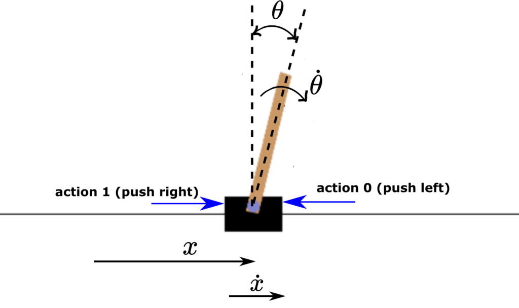
The control objective is to keep the pole in the vertical position by applying horizontal actions (forces) to the cart. The action space consists of two actions

Push the cart left – denoted by 0
Push the cart right – denoted by 1

The observation space or the states are

Cart position, denoted by $x$ in Fig. 1. The minimal and maximal values are -4.8 and 4.8, respectively.
Cart velocity, denoted by $\dot{x}$ in Fig. 1. The minimal and maximal values are $-\infty$ and $\infty$ , respectively.
Pole angle of rotation (measured in radians), denoted by $\theta$ . The minimal and maximal values are -0.418 radians (-24 degrees) and 0.418 (24 degrees).
Pole angular velocity, denoted by $\dot{\theta}$ . The minimal and maximal values are $-\infty$ and $\infty$ , respectively.

Here it is also important to emphasize that initial states (initial observations) are completely random and the values of states are chosen uniformly from the interval (-0.05,0.05).

All observations are assigned a uniformly random value in (-0.05, 0.05)

An episode terminates under the following conditions:

The pole angle becomes greater than |12| degrees (absolute value of $\pm 12$ ) or |0.2095| radians (absolute value of $\pm 0.2095$ ).
Cart position is greater than |2.4| (absolute value of $\pm 2.4$ ).
If the number of steps in an episode is greater than 500 for version v1 of Cart Pole (200 for version v0).

The reward of +1 is obtained every time a step is taken within an episode. This is because the control objective is to keep the pole in the upright position. That is, the higher sum of rewards is obtained for longer episodes (the angle or rotation does not exceed |12| degrees), and when the cart is for a longer time period close the vertical position.

Q-Learning Algorithm

The core of the Q-learning algorithm is an equation for updating the action value function that is denoted by $Q$ . The learning algorithm is summarized below.

Initialize the values of the action value function $Q$ and then loop through the training episodes:

Initialize the environment to the initial state denoted by S
For every time step of a single episode (until the terminal state is reached, that is until the next state S’ is NOT the terminal state):

Step 1: Select action A in the state S on the basis of the epsilon-greedy algorithm.

Step 2: Apply action A to the environment, and observe the reward $R$ and the next state $S'$ .

Step 3: Update the action value function:
– If the next state $S'$ is not the terminal state (S’ is the state that ends the episode)
(1) $\begin{align*} Q(S,A)& \leftarrow Q(S,A) +\alpha \Big(R+\gamma Q_{\text{max}}-Q(S,A) \Big) \\Q_{\text{max}} & =\text{max}_{a} Q(S',a) \end{align*}$

– If the next state $S'$ is the terminal state then $Q(S',A')=0$ by definition, and consequently, update the action value function as follows
(2) $\begin{align*} Q(S,A)& \leftarrow Q(S,A) +\alpha \Big(R-Q(S,A) \Big) \\\end{align*}$

Step 4: Set S=S’ (the current state to the next state) and start again from Step 1.

In the above algorithm, $\alpha>0$ is the step size selected by the user. The parameter $0<\gamma\le 1$ is the discount rate that is also selected by the user. Once the algorithm is executed for a number of episodes, we compute the action value function $Q(S,A)$ . Then, we select the action $A$ in state $S$ simply as

(3) $\begin{align*}A(S)=\text{argmax}_{A}Q(S,A)\end{align*}$

That is, we select the action $A$ in a particular state that produces the maximal value of the action value function at that state.

Here, we also have to have a word or two about the initialization of the Q learning algorithm. Namely, we have to initialize the $Q(S,A)$ for every considered state $S$ and for every action $A$ . In the classical textbook on reinforcement learning

Sutton, R. S., & Barto, A. G. (2018). Reinforcement learning: An introduction. MIT Press.

It is written that $Q(S,A)$ can be initialized arbitrarily, except the values of $Q(S,A)$ for the states $S$ that are the terminal states. If $S$ is a terminal state, then we have the following initialization $Q(S,A)=0$ . However, in the case of the above-stated algorithm, we never actually use $Q(S,A)$ values when the state $S$ is a terminal state. This is because of the two IF statements in step 3 of the algorithm. Consequently, we can completely arbitrarily initialize the algorithm.

Approximation (quantization or discretization)

If the state space (observation space) is completely discrete, then we can apply the Q-learning algorithm without modifications. However, the state space of the Cart Pole system is not discrete. This is because the state row vector

(4) $\begin{align*}S=(x,\dot{x},\theta, \dot{\theta})\end{align*}$

is continuous. This means that any of the state variables $x$ , $\dot{x}$ , $\theta$ , and $\dot{\theta}$ can take any value in the prescribed continuous intervals determined by the limits of the state space. Consequently, since the action value function $Q(S,A)$ is a function of the state, this means that we have an infinite number of action-value functions. Consequently, it is practically impossible to store and update the value of $Q(S,A)$ by using (1). What we want is actually a finite set of action values that can be updated by using the equation (1). That is, we want to approximate a continuous state-space by a finite discrete state-space.

To achieve that, we need to discretize each state variable. For example, let us assume that the state $x$ can be in the interval [0,1]. Then, we can divide this interval into 4 segments:

Segment 0 [0.25]
Segment 1 (0.25,0.5]
Segment 2 (0.5,0.75]
Segment 3 (0.75,1]

The indices of segments start from 0, since we want to be consistent with the Python notation. Then, if for example, x=0.6, we can see that the x belongs to the segment 2. Consequently, we assign

(5) $\begin{align*}x=0.6 \rightarrow \text{discrete index}\; 2\end{align*}$

On the other hand, if $x=0.213$ , we can see that this $x$ belongs to the segment 0. Consequently, we assign

(6) $\begin{align*}x=0.213 \rightarrow \text{discrete index}\; 0\end{align*}$

We can perform this discretization for other state variables. In this way, we can assign to every continuous state vector $S=( x,\dot{x}, \theta,\dot{\theta})$ , a set of discrete indices $(I_{x},I_{\dot{x}},I_{\theta},I_{\dot{\theta}})$ . That is,

(7) $\begin{align*}( x,\dot{x}, \theta,\dot{\theta}) \rightarrow (I_{x},I_{\dot{x}},I_{\theta},I_{\dot{\theta}})\end{align*}$

This discretization process produces the so-called Q-table or Q-matrix shown in the figure below.

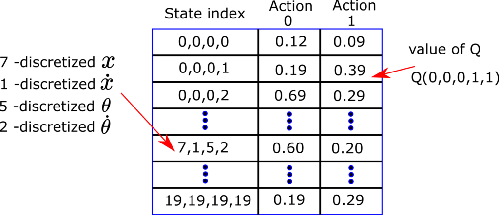
Figure 2: Q-table or Q-matrix obtained by discretizing the states.

For the fixed continuous state $S=( x,\dot{x}, \theta,\dot{\theta})$ and for the fixed action, we can assign the value of $Q$ . For example, $Q(0,0,0,1,1)$ , is the Q value for the discretized state index $(0,0,0,1)$ and for the action $1$ .

By using the Q-table we can run the algorithm. First, we observe the state $S$ , then, we discretize this state, to obtain discrete indices $(I_{x},I_{\dot{x}},I_{\theta},I_{\dot{\theta}})$ . Then, we can use these discrete indices to select a row of the Q-table, that represents the action value function values for certain actions. By using this type of discretization and indexing we can run the Q-learning algorithm.

Python Codes Implementing the Q-Learning Algorithm

Here, we present Python codes that implement the Q-Learning algorithm. We wrote a class called Q_Learning that implements:

Q-Learning algorithm
Simulation of the optimal learned policy
Simulation of random policies

We wrote code that simulates the random policies in order to establish a baseline for evaluating the optimal learned policy.

import numpy as np

class Q_Learning:
    ###########################################################################
    #   START - __init__ function
    ###########################################################################
    # INPUTS: 
    # env - Cart Pole environment
    # alpha - step size 
    # gamma - discount rate
    # epsilon - parameter for epsilon-greedy approach
    # numberEpisodes - total number of simulation episodes
    
    # numberOfBins - this is a 4 dimensional list that defines the number of grid points 
    # for state discretization
    # that is, this list contains number of bins for every state entry, 
    # we have 4 entries, that is,
    # discretization for cart position, cart velocity, pole angle, and pole angular velocity
    
    # lowerBounds - lower bounds (limits) for discretization, list with 4 entries:
    # lower bounds on cart position, cart velocity, pole angle, and pole angular velocity

    # upperBounds - upper bounds (limits) for discretization, list with 4 entries:
    # upper bounds on cart position, cart velocity, pole angle, and pole angular velocity
    
    def __init__(self,env,alpha,gamma,epsilon,numberEpisodes,numberOfBins,lowerBounds,upperBounds):
        import numpy as np
        
        self.env=env
        self.alpha=alpha
        self.gamma=gamma 
        self.epsilon=epsilon 
        self.actionNumber=env.action_space.n 
        self.numberEpisodes=numberEpisodes
        self.numberOfBins=numberOfBins
        self.lowerBounds=lowerBounds
        self.upperBounds=upperBounds
        
        # this list stores sum of rewards in every learning episode
        self.sumRewardsEpisode=[]
        
        # this matrix is the action value function matrix 
        self.Qmatrix=np.random.uniform(low=0, high=1, size=(numberOfBins[0],numberOfBins[1],numberOfBins[2],numberOfBins[3],self.actionNumber))
        
    
    ###########################################################################
    #   END - __init__ function
    ###########################################################################
    
    ###########################################################################
    # START: function "returnIndexState"
    # for the given 4-dimensional state, and discretization grid defined by 
    # numberOfBins, lowerBounds, and upperBounds, this function will return 
    # the index tuple (4-dimensional) that is used to index entries of the 
    # of the QvalueMatrix 


    # INPUTS:
    # state - state list/array, 4 entries: 
    # cart position, cart velocity, pole angle, and pole angular velocity

    # OUTPUT: 4-dimensional tuple defining the indices of the QvalueMatrix 
    # that correspond to "state" input

    ###############################################################################
    def returnIndexState(self,state):
        position =      state[0]
        velocity =      state[1]
        angle    =      state[2]
        angularVelocity=state[3]
        
        cartPositionBin=np.linspace(self.lowerBounds[0],self.upperBounds[0],self.numberOfBins[0])
        cartVelocityBin=np.linspace(self.lowerBounds[1],self.upperBounds[1],self.numberOfBins[1])
        poleAngleBin=np.linspace(self.lowerBounds[2],self.upperBounds[2],self.numberOfBins[2])
        poleAngleVelocityBin=np.linspace(self.lowerBounds[3],self.upperBounds[3],self.numberOfBins[3])
        
        indexPosition=np.maximum(np.digitize(state[0],cartPositionBin)-1,0)
        indexVelocity=np.maximum(np.digitize(state[1],cartVelocityBin)-1,0)
        indexAngle=np.maximum(np.digitize(state[2],poleAngleBin)-1,0)
        indexAngularVelocity=np.maximum(np.digitize(state[3],poleAngleVelocityBin)-1,0)
        
        return tuple([indexPosition,indexVelocity,indexAngle,indexAngularVelocity])   
    ###########################################################################
    #   END - function "returnIndexState"
    ###########################################################################    
       
    ###########################################################################
    #    START - function for selecting an action: epsilon-greedy approach
    ###########################################################################
    # this function selects an action on the basis of the current state 
    # INPUTS: 
    # state - state for which to compute the action
    # index - index of the current episode
    def selectAction(self,state,index):
        
        # first 500 episodes we select completely random actions to have enough exploration
        if index<500:
            return np.random.choice(self.actionNumber)   
            
        # Returns a random real number in the half-open interval [0.0, 1.0)
        # this number is used for the epsilon greedy approach
        randomNumber=np.random.random()
        
        # after 7000 episodes, we slowly start to decrease the epsilon parameter
        if index>7000:
            self.epsilon=0.999*self.epsilon
        
        # if this condition is satisfied, we are exploring, that is, we select random actions
        if randomNumber < self.epsilon:
            # returns a random action selected from: 0,1,...,actionNumber-1
            return np.random.choice(self.actionNumber)            
        
        # otherwise, we are selecting greedy actions
        else:
            # we return the index where Qmatrix[state,:] has the max value
            # that is, since the index denotes an action, we select greedy actions
            return np.random.choice(np.where(self.Qmatrix[self.returnIndexState(state)]==np.max(self.Qmatrix[self.returnIndexState(state)]))[0])
            # here we need to return the minimum index since it can happen
            # that there are several identical maximal entries, for example 
            # import numpy as np
            # a=[0,1,1,0]
            # np.where(a==np.max(a))
            # this will return [1,2], but we only need a single index
            # that is why we need to have np.random.choice(np.where(a==np.max(a))[0])
            # note that zero has to be added here since np.where() returns a tuple
    ###########################################################################
    #    END - function selecting an action: epsilon-greedy approach
    ###########################################################################
    
    
    ###########################################################################
    #    START - function for simulating learning episodes
    ###########################################################################
     
    def simulateEpisodes(self):
        import numpy as np
        # here we loop through the episodes
        for indexEpisode in range(self.numberEpisodes):
            
            # list that stores rewards per episode - this is necessary for keeping track of convergence 
            rewardsEpisode=[]
            
            # reset the environment at the beginning of every episode
            (stateS,_)=self.env.reset()
            stateS=list(stateS)
          
            print("Simulating episode {}".format(indexEpisode))
            
            
            # here we step from one state to another
            # this will loop until a terminal state is reached
            terminalState=False
            while not terminalState:
                # return a discretized index of the state
                
                stateSIndex=self.returnIndexState(stateS)
                
                # select an action on the basis of the current state, denoted by stateS
                actionA = self.selectAction(stateS,indexEpisode)
                
                
                # here we step and return the state, reward, and boolean denoting if the state is a terminal state
                # prime means that it is the next state
                (stateSprime, reward, terminalState,_,_) = self.env.step(actionA)          
                
                rewardsEpisode.append(reward)
                
                stateSprime=list(stateSprime)
                
                stateSprimeIndex=self.returnIndexState(stateSprime)
                
                # return the max value, we do not need actionAprime...
                QmaxPrime=np.max(self.Qmatrix[stateSprimeIndex])                                               
                                             
                if not terminalState:
                    # stateS+(actionA,) - we use this notation to append the tuples
                    # for example, for stateS=(0,0,0,1) and actionA=(1,0)
                    # we have stateS+(actionA,)=(0,0,0,1,0)
                    error=reward+self.gamma*QmaxPrime-self.Qmatrix[stateSIndex+(actionA,)]
                    self.Qmatrix[stateSIndex+(actionA,)]=self.Qmatrix[stateSIndex+(actionA,)]+self.alpha*error
                else:
                    # in the terminal state, we have Qmatrix[stateSprime,actionAprime]=0 
                    error=reward-self.Qmatrix[stateSIndex+(actionA,)]
                    self.Qmatrix[stateSIndex+(actionA,)]=self.Qmatrix[stateSIndex+(actionA,)]+self.alpha*error
                
                # set the current state to the next state                    
                stateS=stateSprime
        
            print("Sum of rewards {}".format(np.sum(rewardsEpisode)))        
            self.sumRewardsEpisode.append(np.sum(rewardsEpisode))
 
        
    ###########################################################################
    #    END - function for simulating learning episodes
    ###########################################################################
    
    
    ###########################################################################
    #    START - function for simulating the final learned optimal policy
    ###########################################################################
    # OUTPUT: 
    # env1 - created Cart Pole environment
    # obtainedRewards - a list of obtained rewards during time steps of a single episode
    
    # simulate the final learned optimal policy
    def simulateLearnedStrategy(self):
        import gym 
        import time
        env1=gym.make('CartPole-v1',render_mode='human')
        (currentState,_)=env1.reset()
        env1.render()
        timeSteps=1000
        # obtained rewards at every time step
        obtainedRewards=[]
        
        for timeIndex in range(timeSteps):
            print(timeIndex)
            # select greedy actions
            actionInStateS=np.random.choice(np.where(self.Qmatrix[self.returnIndexState(currentState)]==np.max(self.Qmatrix[self.returnIndexState(currentState)]))[0])
            currentState, reward, terminated, truncated, info =env1.step(actionInStateS)
            obtainedRewards.append(reward)   
            time.sleep(0.05)
            if (terminated):
                time.sleep(1)
                break
        return obtainedRewards,env1
    ###########################################################################
    #    END - function for simulating the final learned optimal policy
    ###########################################################################     
                 
    ###########################################################################
    #    START - function for simulating random actions many times
    #   this is used to evaluate the optimal policy and to compare it with a random policy
    ###########################################################################
    #  OUTPUT:
    # sumRewardsEpisodes - every entry of this list is a sum of rewards obtained by simulating the corresponding episode
    # env2 - created Cart Pole environment
    def simulateRandomStrategy(self):
        import gym 
        import time
        import numpy as np
        env2=gym.make('CartPole-v1')
        (currentState,_)=env2.reset()
        env2.render()
        # number of simulation episodes
        episodeNumber=100
        # time steps in every episode
        timeSteps=1000
        # sum of rewards in each episode
        sumRewardsEpisodes=[]
        
        
        for episodeIndex in range(episodeNumber):
            rewardsSingleEpisode=[]
            initial_state=env2.reset()
            print(episodeIndex)
            for timeIndex in range(timeSteps):
                random_action=env2.action_space.sample()
                observation, reward, terminated, truncated, info =env2.step(random_action)
                rewardsSingleEpisode.append(reward)
                if (terminated):
                    break      
            sumRewardsEpisodes.append(np.sum(rewardsSingleEpisode))
        return sumRewardsEpisodes,env2
    ###########################################################################
    #    END - function for simulating random actions many times
    ###########################################################################

The “init” function on the code lines 26 to 43 initializes the parameters of the learning algorithm. It accepts the following input parameters:

“env” – this is the Cart Pole OpenAI Gym environment.
“alpha” is the parameter $\alpha$ (step size)
“gamma” is the parameter $\gamma$ (discount rate)
“epsilon” is the parameter $\varepsilon$ of the epsilon-greedy algorithm. For more details see the explanation of the epsilon greedy algorithm given here.
“numberEpisodes” is the number of simulation (learning) episodes of the Q-Learning algorithm.
“numberOfBins” is the 1 by 4 vector (list) defining the number of discretization points for state variables $x$ , $\dot{x}$ , $\theta$ , and $\dot{\theta}$ (see the comment below).
“lowerBounds” – is the 1 by 4 vector (list) defining the lower bounds for the state variables $x$ , $\dot{x}$ , $\theta$ , and $\dot{\theta}$ . This lower bound is used in the discretization process (see the comment below).
“upperBounds” – is the 1 by 4 vector (list) defining the upper bounds for the state variables $x$ , $\dot{x}$ , $\theta$ , and $\dot{\theta}$ . This lower bound is used in the discretization process (see the comment below).

Comment: The discretization grid starts from values given in “lowerBounds” and ends at the values in “upperBounds”. The numbers of discretization points between these bounds are given in “numberOfBins” for each state variable.

The initialized list “sumRewardsEpisode” is used to store the obtained rewards during each training episode. The initialized multi-dimensional matrix “Qmatrix” is used to store the Q matrix. That is, it is used to store the values of the action value function. We initialize the values of this matrix as random real numbers.

The function “returnIndexState()” defined in the code lines 66 to 82 is used to discretize the state. It accepts the state vector ( $x$ , $\dot{x}$ , $\theta$ , and $\dot{\theta}$ ), and returns a discrete index (tuple) that is used to access the entries of the matrix Qmatrix.

The function “selectAction()” defined in the code lines 94 to 128, implements the epsilon-greedy method explained here. Note here that during the first 500 training episodes we are only exploring the environment by selecting random actions.

The function “simulateEpisodes” defined in the code lines 135 to 190 is used to learn the optimal policy. It loops through the learning (training episodes) and it updates the entries of Qmatrix by using the Q-Learning algorithm.

The function “simulateLearnedStrategy” defined in the code lines 206 to 227 is used to simulate the final optimal learned policy.

The function “simulateRandomStrategy” defined in the code lines 238 to 264 is used to simulate a random policy. This function is used to provide a baseline for comparing the optimal learned policy with a purely random policy.

The driver code for the defined class is given below.

# Note: 
# You can either use gym (not maintained anymore) or gymnasium (maintained version of gym)    
    
# tested on     
# gym==0.26.2
# gym-notices==0.0.8

#gymnasium==0.27.0
#gymnasium-notices==0.0.1

# classical gym 
import gym
# instead of gym, import gymnasium 
# import gymnasium as gym
import numpy as np
import time
import matplotlib.pyplot as plt 

# import the class that implements the Q-Learning algorithm
from functions import Q_Learning

#env=gym.make('CartPole-v1',render_mode='human')
env=gym.make('CartPole-v1')
(state,_)=env.reset()
#env.render()
#env.close()

# here define the parameters for state discretization
upperBounds=env.observation_space.high
lowerBounds=env.observation_space.low
cartVelocityMin=-3
cartVelocityMax=3
poleAngleVelocityMin=-10
poleAngleVelocityMax=10
upperBounds[1]=cartVelocityMax
upperBounds[3]=poleAngleVelocityMax
lowerBounds[1]=cartVelocityMin
lowerBounds[3]=poleAngleVelocityMin

numberOfBinsPosition=30
numberOfBinsVelocity=30
numberOfBinsAngle=30
numberOfBinsAngleVelocity=30
numberOfBins=[numberOfBinsPosition,numberOfBinsVelocity,numberOfBinsAngle,numberOfBinsAngleVelocity]

# define the parameters
alpha=0.1
gamma=1
epsilon=0.2
numberEpisodes=15000

# create an object
Q1=Q_Learning(env,alpha,gamma,epsilon,numberEpisodes,numberOfBins,lowerBounds,upperBounds)
# run the Q-Learning algorithm
Q1.simulateEpisodes()
# simulate the learned strategy
(obtainedRewardsOptimal,env1)=Q1.simulateLearnedStrategy()

plt.figure(figsize=(12, 5))
# plot the figure and adjust the plot parameters
plt.plot(Q1.sumRewardsEpisode,color='blue',linewidth=1)
plt.xlabel('Episode')
plt.ylabel('Reward')
plt.yscale('log')
plt.show()
plt.savefig('convergence.png')


# close the environment
env1.close()
# get the sum of rewards
np.sum(obtainedRewardsOptimal)

# now simulate a random strategy
(obtainedRewardsRandom,env2)=Q1.simulateRandomStrategy()
plt.hist(obtainedRewardsRandom)
plt.xlabel('Sum of rewards')
plt.ylabel('Percentage')
plt.savefig('histogram.png')
plt.show()

# run this several times and compare with a random learning strategy
(obtainedRewardsOptimal,env1)=Q1.simulateLearnedStrategy()

First, in the code lines 11 to 20 we import the necessary libraries and class definitions. Then, in the code lines 22 to 50 we define the parameters of the algorithm. Then, in the code line 53, we create an object $Q1$ that is used to simulate the Q-Learning algorithm. Then, we run the learning process by executing Q1.simulateEpisodes(). This code line will start the learning process. After the learning process is completed, we call the function Q1.simulateEpisodes() to simulate the final learned strategy. After this code line is executed, a simulation window will appear with animation showing the effect of the final optimal strategy.

We plot the sum of rewards obtained in every learning episode in the code lines 59 to 66. The results are given in the figure below.

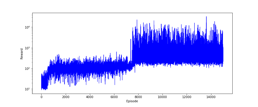
Fig 2: Rewards obtained during the learning episodes.

We can observe that gradually the sum of rewards increases during episodes.

Finally, we compare the optimal learned policy with a random policy by executing the code line 75. The figure below shows a histogram of the sum of rewards obtained by using a random strategy.

Fig. 3: Histogram of the sum of rewards obtained by using a random strategy

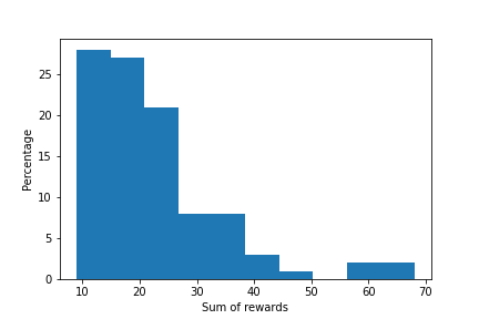
We run the optimal learned strategy many times. Every time, we obtained a different value of the sum of rewards. This is because in every episode simulation, the system is initialized from a different initial state. By running 5 simulations of the optimal learning strategy, we obtained the sum rewards of 345, 521, 687, 635, and 451

We can observe that the optimal learning policy obtains a much higher sum of rewards compared to the random learning strategy. This is clear evidence that the Q-Learning algorithm works in practice.

Prerequisites and Cart Pole Environment

Q-Learning Algorithm

Approximation (quantization or discretization)

Python Codes Implementing the Q-Learning Algorithm

admin

You might also like

Control of Drone and Quadrotor DC Motors by Using Teensy/Arduino and PWM Signals

Implement Newton’s Method in Python From Scratch by Using SymPy Symbolic Toolbox and Automatic Differentiation

High-School and Undergraduate Student Tutoring, Mentoring, and Academic Coaching in Orange County, Irvine, and Los Angeles