In this post, we derive equations describing the recursive least squares method. The motivation for creating this tutorial, comes from the fact that these equations are used in the derivation of the Kalman filter equations. Apart from this, the recursive least squares method is the basis of many other algorithms, such as adaptive control algorithms. Consequently, it is of paramount importance to properly understand the recursive least-squares method. The derivation of the Kalman filter equations on the basis of the recursive least-squares equations is arguably much simpler and easier to understand than the derivation based on other methods or approaches.
The Python implementation of the derived least-squares method is given here.
The YouTube videos accompanying this post are given below.
Motivational Example
To motivate the need for the recursive least squares method, we consider the following example. We assume that a vehicle is moving from a starting position ![]() , with an initial velocity, denoted by
, with an initial velocity, denoted by ![]() , and with an acceleration denoted by
, and with an acceleration denoted by ![]() . Our goal is to estimate,
. Our goal is to estimate, ![]() ,
, ![]() , and
, and ![]() , by only measuring position values
, by only measuring position values ![]() obtained by a distance sensor. Here,
obtained by a distance sensor. Here, ![]() denotes the time variable. From the basic kinematics equations that relate the position, velocity, and acceleration, we know that the following model fully kinematically describes the motion of the car
denotes the time variable. From the basic kinematics equations that relate the position, velocity, and acceleration, we know that the following model fully kinematically describes the motion of the car
(1) ![]()
We assume that we are able to measure the position at the discrete-time instants ![]() , where
, where ![]() is the sampling period of the sensor. Next, let
is the sampling period of the sensor. Next, let ![]() . Our measurement equation is then
. Our measurement equation is then
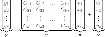
(2) 
where ![]() is the measurement noise. Clearly, our
is the measurement noise. Clearly, our ![]() matrix is then
matrix is then
(3) ![]()
And our vector ![]() is then
is then
(4) 
The goal of the recursive least squares method is to estimate the vector ![]() recursively on the basis of the sequentially obtained data
recursively on the basis of the sequentially obtained data ![]() . That is, we start from some initial guess of
. That is, we start from some initial guess of ![]() , denoted by
, denoted by ![]() . When the initial measurement sample
. When the initial measurement sample ![]() arrives, we should update the initial estimate. Then, when the next sample
arrives, we should update the initial estimate. Then, when the next sample ![]() arrives, we should use this sample to update the previously computed estimate. This procedure is repeated every time a new measurement sample arrives.
arrives, we should use this sample to update the previously computed estimate. This procedure is repeated every time a new measurement sample arrives.
Issues with the ordinary least squares method
In our previous post which can be found here, we derived the solution to the least squares problem. Here for completeness of this tutorial, we briefly revise the ordinary least squares method.
Consider the following system of linear equations
(5) 
where ![]() ,
, ![]() are real scalar variables that we want to determine (unknowns),
are real scalar variables that we want to determine (unknowns), ![]() are scalars and
are scalars and ![]() is the measurement noise. The noise term is not known. However, we assume that we know the statistical properties of the noise that can be estimated from the data. We assume that the measurement noise is zero mean and that
is the measurement noise. The noise term is not known. However, we assume that we know the statistical properties of the noise that can be estimated from the data. We assume that the measurement noise is zero mean and that
(6) ![]()
where ![]() is an expectation operator and
is an expectation operator and ![]() is a variance (
is a variance (![]() is a standard deviation) . Furthermore, we assume that
is a standard deviation) . Furthermore, we assume that ![]() and
and ![]() are statistically independent for all
are statistically independent for all ![]() .
.
The equations in (5) can be compactly written as follows
(7) 
where ![]() and
and ![]() . In (7) and throughout this post, vector quantities are denoted using a bold font. The last equation can be compactly written as follows:
. In (7) and throughout this post, vector quantities are denoted using a bold font. The last equation can be compactly written as follows:
(8) ![]()
Usually, in the least squares estimation problems ![]() , that is, the number of measurements
, that is, the number of measurements ![]() is usually much larger than the number of variables to be estimated. Under the assumption that the matrix
is usually much larger than the number of variables to be estimated. Under the assumption that the matrix ![]() has a full column rank and under the assumption that
has a full column rank and under the assumption that ![]() , the least squares solution is found by solving the following optimization problem
, the least squares solution is found by solving the following optimization problem
(9) ![]()
There are a number of computationally efficient approaches for solving (9). Here for brevity and simplicity, we use the solution that is not the most efficient one to be computed. This solution is given by the following equation
(10) ![]()
There are at least two issues with the formulation and solution of the least squares problem:
- The least-squares problem formulation and its solutions assume that all measurements are available at a certain time instant. However, this often might not be the case in the practice. Also, we would like to update the solution as new measurements arrive in order to have an adaptive approach for updating the solution.
- When the number of measurements
 is extremely large, the solutions of the least squares problem are difficult to compute. That is, the computational and memory complexities of the solution are very high.
These facts motivate the development of the recursive least squares that is presented in the sequel.
Recursive Least Squares Method – Complete Derivation From Scratch
Let us assume that at the discrete-time instant ![]() , the set of measurements grouped in the vector
, the set of measurements grouped in the vector ![]() becomes available. Let us assume that these measurements are related to the vector
becomes available. Let us assume that these measurements are related to the vector ![]() that we want to estimate by the following equation
that we want to estimate by the following equation
(11) ![]()
where ![]() , and
, and ![]() is the measurement noise vector. We assume that the covariance of the measurement noise is given by
is the measurement noise vector. We assume that the covariance of the measurement noise is given by
(12) ![]()
and we assume that the mean of ![]() is zero:
is zero:
(13) ![]()
The recursive least-squares method that we derive in this section, has the following form:
(14) ![]()
where ![]() and
and ![]() are the estimates of the vector
are the estimates of the vector ![]() at the discrete-time instants
at the discrete-time instants ![]() and
and ![]() , and
, and ![]() is the gain matrix that we need to determine.
is the gain matrix that we need to determine.
The equation (14) updates the estimate of ![]() at the time instant
at the time instant ![]() on the basis of the estimate
on the basis of the estimate ![]() at the previous time instant
at the previous time instant ![]() and on the basis of the measurement
and on the basis of the measurement ![]() obtained at the time instant
obtained at the time instant ![]() , as well as on the basis of the gain matrix
, as well as on the basis of the gain matrix ![]() computed at the time instant
computed at the time instant ![]() .
.
Our goal is to derive the formulas for computing the gain matrix ![]() .
.
First, we need to introduce new notation. We assume that the vector ![]() is partitioned as follows
is partitioned as follows
(15) 
This partitioning directly corresponds to the partitioning of the vector ![]()
(16) 
Next, we introduce the estimation error vector ![]() and the following partitioning:
and the following partitioning:
(17) 
That is,
(18) ![]()
The gain ![]() is computed by minimizing the sum of variances of the estimation errors
is computed by minimizing the sum of variances of the estimation errors
(19) ![]()
Next, we show that this cost function, can be represented as follows:
(20) ![]()
where ![]() is the notation for the matrix trace, and
is the notation for the matrix trace, and ![]() is the estimation error covariance matrix that is defined by
is the estimation error covariance matrix that is defined by
(21) ![]()
That is, the gain matrix ![]() is found by minimizing the trace of the estimation error covariance matrix.
is found by minimizing the trace of the estimation error covariance matrix.
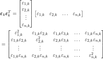
To show this, let us first expand the following expression
(22) 
From the last expression, we have
(23) ![Rendered by QuickLaTeX.com \begin{align*}P_{k}& = E[\boldsymbol{\varepsilon}_{k}\boldsymbol{\varepsilon}^{T}_{k}] \\& = \begin{bmatrix} E[\varepsilon_{1,k}^{2}] & E[\varepsilon_{1,k}\varepsilon_{2,k}] & E[\varepsilon_{1,k}\varepsilon_{3,k}] & \ldots & E[\varepsilon_{1,k}\varepsilon_{n,k}] \\ E[\varepsilon_{1,k}\varepsilon_{2,k}] & E[\varepsilon_{2,k}^{2}] & E[\varepsilon_{2,k}\varepsilon_{3,k}] & \ldots & E[\varepsilon_{2,k}\varepsilon_{n,k}] \\ \vdots & \vdots & \vdots & \hdots & \vdots \\ E[\varepsilon_{1,k}\varepsilon_{n,k}] & E[\varepsilon_{2,k}\varepsilon_{n,k}] &E[\varepsilon_{3,k}\varepsilon_{n,k}] & \ldots & E[\varepsilon_{n,k}^{2}] \end{bmatrix}\end{align*}](https://aleksandarhaber.com/wp-content/ql-cache/quicklatex.com-6daf621a35f60868f801a88ba235403e_l3.png)
Next, by taking the matrix trace of the last expression, we obtain
(24) ![]()
and this is exactly the expression for the cost function ![]() given by (19).
given by (19).
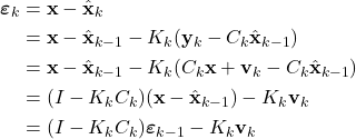
Next, we derive the expression for the time propagation of the estimation covariance matrix. By substituting the estimate propagation equation (14) and the measurement equation (11) in the expression for the estimation error, we obtain
(25) 
Next, we have
(26) 
Applying the expectation operator to (26), we obtain
(27) ![Rendered by QuickLaTeX.com \begin{align*}P_{k} & =E[\boldsymbol{\varepsilon}_{k}\boldsymbol{\varepsilon}^{T}_{k}] \\& = (I-K_{k}C_{k})E[\boldsymbol{\varepsilon}_{k-1}\boldsymbol{\varepsilon}^{T}_{k-1}](I-K_{k}C_{k})^{T}-(I-K_{k}C_{k})E[\boldsymbol{\varepsilon}_{k-1}\mathbf{v}_{k}^{T}]K_{k}^{T} \\& -K_{k}E[\mathbf{v}_{k}\boldsymbol{\varepsilon}^{T}_{k-1}](I-K_{k}C_{k})^{T}+K_{k}E[\mathbf{v}_{k}\mathbf{v}_{k}^{T}]K_{k}^{T}\end{align*}](https://aleksandarhaber.com/wp-content/ql-cache/quicklatex.com-667aae12e34ce65e1047c2a750709110_l3.png)
We have
(28) ![]()
Then, since ![]() and
and ![]() are independent (measurement noise at the time instant
are independent (measurement noise at the time instant ![]() is independent from the estimation error at the time instant
is independent from the estimation error at the time instant ![]() ), and due to the fact that
), and due to the fact that ![]() is zero-mean:
is zero-mean:
(29) ![]()
(30) ![]()
(31) ![]()
By substituting (28), (29), (30), and (31) in (27), we obtain an important expression for the propagation of the estimation error covariance matrix
(32) ![]()
Let us expand the last expression
(33) ![]()
By substituting (49) in (20), we obtain
(34) 
We find the gain matrix ![]() by optimizing the cost function (34). That is, we find the value of
by optimizing the cost function (34). That is, we find the value of ![]() by solving the following equation
by solving the following equation
(35) ![]()
To compute the derivatives of matrix traces, we use the formulas given in The Matrix Cookbook (Section 2.5). We use the following formulas
(36) ![]()
(37) ![]()
(38) ![]()
We find derivatives of all terms in (34). Since ![]() is constant, we have
is constant, we have
(39) ![]()
Next, by using (36), we have
(40) ![]()
By using (37), we have
(41) ![]()
By using (38), we have
(42) ![]()
(43) ![]()
By substituting (39), (40), (41), (42), and (43):
(44) ![]()
From the last equation, we have
(45) ![]()
By solving the last equation we obtain the final expression for the gain matrix ![]()
(46) ![]()
Before we summarize the recursive least-squares method, we derive an alternative form of the estimation error covariance matrix propagation equation. First, we can write the gain matrix (46), as follows
(47) ![]()
Here, we should observe that the matrix ![]() and its inverse
and its inverse ![]() are symmetric, that is
are symmetric, that is
(48) ![]()
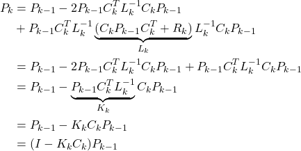
We substitute (47) in (49), and as the result, we obtain
(49) 
By adding the second and third terms and by grouping the last two terms, we obtain
(50) 
That is, an alternative expression for the propagation of the estimation error covariance matrix is given by
(51) ![]()
Consequently, the recursive least squares method consists of the following three equations
- Gain matrix update
(52)

- Estimate update
(53)

- Propagation of the estimation error covariance matrix by using this equation
(54)

or this equation(55)

If no apriori knowledge of the estimate is known, then this method is initialized with the estimation error covariance matrix that is equal to , where
  is a large number, and with a random value of
  .
.
The Python implementation of the derived least-squares method is given here.