Simulate Control Systems with Actuator Limits in Simulink – Introduction to Simulink Simulation – Fusion of Engineering, Control, Coding, Machine Learning, and Science

In this post and the accompanying video, we explain how to simulate a control system with actuator constraints in Simulink. The YouTube video accompanying this post is given below.

The Simulink model is given below. If you cannot see this graph clearly, please open the YouTube video, where this diagram is explained.

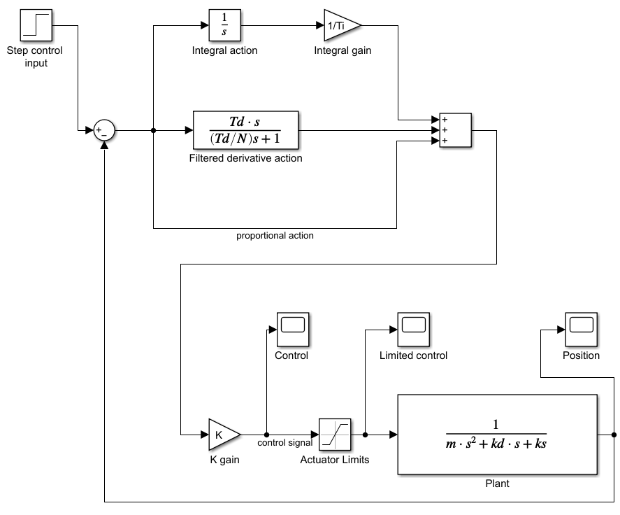
Figure 1: Simulink model of the closed-loop system.

This Simulink block diagram simulates the PID control algorithm having the following form

(1) $\begin{align*}C(s)=K\Big(1+\frac{1}{sT_{i}}+\frac{sT_{d}}{1+s\big(\frac{T_{d}}{N}\big)} \Big)\end{align*}$

where

$C(s)$ is the controller transfer function
$K,T_{i},T_{d},N$ – are the controller constants that are used as tuning parameters
$s$ is the Laplace transform

This form of the PID controller is based on replacing the ideal derivative term $T_{d} s$ by its filtered version

(2) $\begin{align*}\frac{sT_{d}}{1+s\big(\frac{T_{d}}{N}\big)}\end{align*}$

This filtered derivative action acts as a derivative for low-frequency signals, while for the high-frequency signals it acts as a low-pass filter. In this way, we can avoid the amplification of high-frequency signal components by the pure derivative action.

The plan mode is a mass-spring-damper system, described by the following differential equation

(3) $\begin{align*}m\ddot{x}+k_{d}\dot{x}+k_{s}x=F\end{align*}$

where

$m$ is the mass
$k_{d}$ is the damping constant
$k_{s}$ is the spring constant
F is the applied force

The transfer function corresponding to this model is given by

(4) $\begin{align*}W(s)=\frac{X(s)}{F(s)}=\frac{1}{ms^{2}+k_{d}s+k_{s}}\end{align*}$

In reality, the control actuators cannot exert an infinite amount of force. To take this constraint into account, we add the actuator limits to the system model. The actuator limits are shown in Figure 1.

The purpose of this tutorial is not to explain how to tune the PID controllers. Instead, we mainly focus on explaining how to simulate the system behavior. We simulate the system behavior for the following parameters:

$m=30$ , $k_{d}=5$ , $k_{s}=10$ , $T_{i}=20$ , $T_{d}=0.1$ , $N=10$ , and $K=1000$ , and we set the actuator limits to -100 and 100. Also, the step input signal is equal to 1.

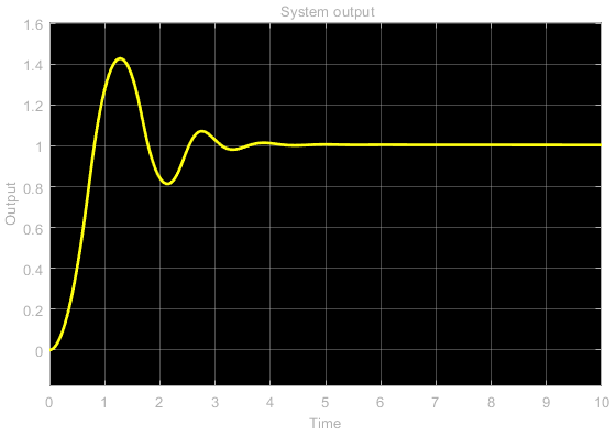
The output of the closed-loop system is shown in the figure below. This graph is obtained by using the probe “Position” in the Simulink diagram.

The control signal that is a direct output of the control algorithm is shown in the figure below. This signal is obtained by using the probe “Control” in the Simulink diagram.

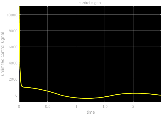
We can see that this output has large values. However, in practice, we cannot achieve these large values. These values are filtered through the actuator limit filter. The limited signal that is applied to the system is shown in the figure below. Note that this signal is obtained by the probe “Limited control”.

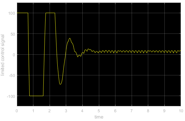
From Fig. 3, we can observe the effect of the actuator saturation.

admin

You might also like

Phase Lead Compensator – Derivation of Equations and Design Procedure

Time Propagation of State Vector Expectation and State Covariance Matrix of Linear Dynamical Systems – Intro to Kalman Filtering

Simulation of Ordinary Differential Equations (ODEs) with Time-varying Coefficients and Time-varying Inputs in MATLAB