Implementing Perceptron Neural Network for Classification in Python – Fusion of Engineering, Control, Coding, Machine Learning, and Science

In this post, we explain how to implement the perceptron neural network for classification tasks from scratch.

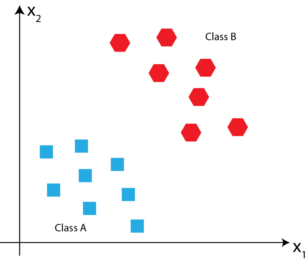
To motivate the need for perceptron, let us consider the following problem. Suppose that we are given two sets of points in the X_{1}-X_{2} planes:

(1) $\begin{align*}\text{Class A}= \{(x_{1}^{A1},x_{2}^{A1}),(x_{1}^{A2},x_{2}^{A2}),\ldots, (x_{1}^{AN},x_{2}^{AN})\} \\\text{Class B}= \{(x_{1}^{B1},x_{2}^{B1}),(x_{1}^{B2},x_{2}^{B2}),\ldots, (x_{1}^{BM},x_{2}^{BM})\} \end{align*}$

where $N$ and $M$ are the numbers of points in the ClassA and ClassB. For example, these two classes are shown in Fig. 1 below.

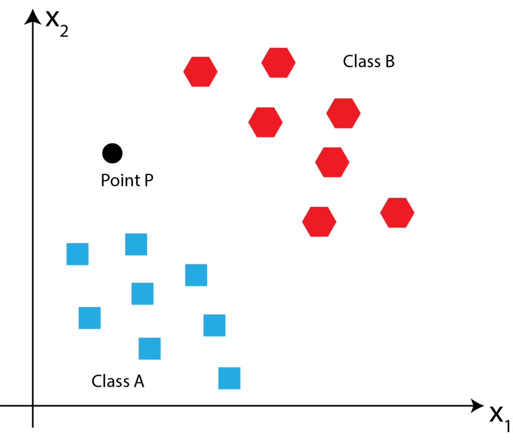
Figure 1: Two classes: Class A (rectangle) and Class B (polygon).

Now, suppose that we are given a new point P: $(x_{1}^{P},x_{2}^{P} )$ . Our task is to determine if this point belongs to Class A or Class B? Point P is illustrated in the figure below.

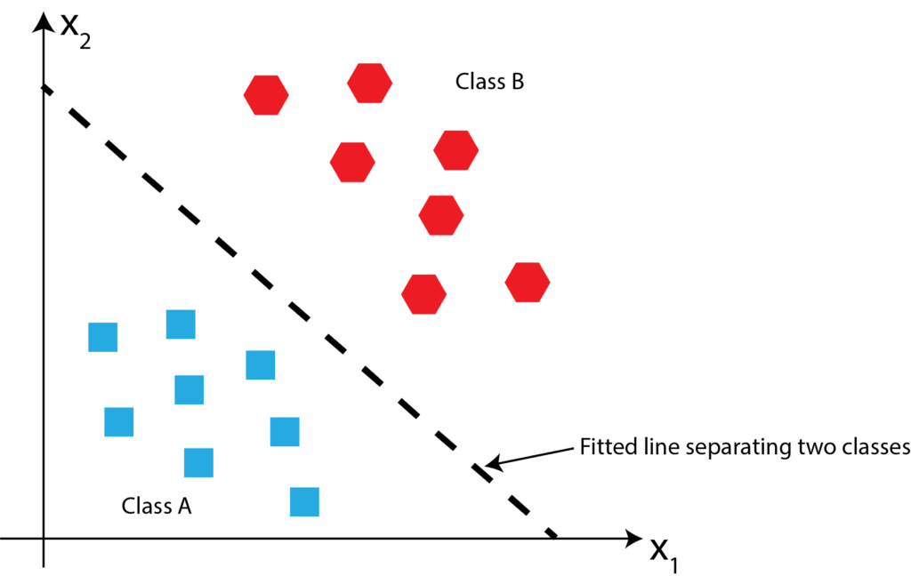
Figure 2: The goal is to determine if new point P belongs to class A or class B.

One way to solve this problem is to first fit the line that will separate these two classes, then once this line is fitted, we can easily determine where the point P belongs by investigating if the point P is above or below the fitted line. The fitted line is shown in the figure below.

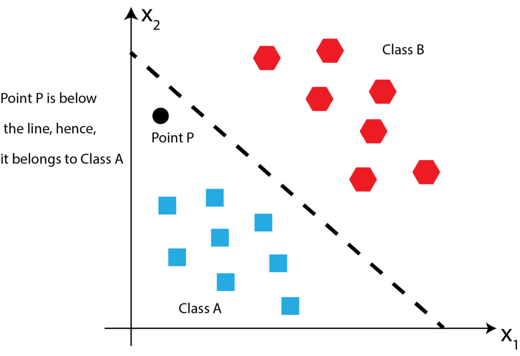
Figure 3: The fitted line separating two classes.

Since point P is below the fitted line, it belongs to class P. This is shown in the figure below.

Let us mathematically formulate this problem and explain how to solve it. First, let us define the line. In the general case, the line will have the following canonical form

(2) $\begin{align*}0=w_{0}x_{0}+w_{1}x_{1}+w_{2}x_{2}+\ldots +w_{q}x_{q}\end{align*}$

where $w_{i}$ , $i=0,1,2,\ldots, q$ are the weights that need to be determined, $x_{0}=1$ by default, and $x_{i}$ , $i=1,2,\ldots, q$ are called the features in the machine learning terminology. The weight $w_{0}$ is called the bias weight, and its corresponding feature is set to $1$ by default. Here, we have assumed the general case for $q$ input features. For example, in Figs. 1-4, the situation is shown for q=2.

With the line (2), we associate the net input function

(3) $\begin{align*}z=w_{0}x_{0}+w_{1}x_{1}+w_{2}x_{2}+\ldots +w_{q}x_{q}\end{align*}$

This function can also be written in the vector form

(4) $\begin{align*}z=\mathbf{w}^{T}\cdot \mathbf{x}\end{align*}$

where

(5) $\begin{align*}\mathbf{w}=\begin{bmatrix}w_{0}\\ w_{1}\\ \vdots \\ w_{q} \end{bmatrix}, \;\; \mathbf{x}=\begin{bmatrix} x_{0}\\x_{1}\\ \vdots \\ x_{q} \end{bmatrix}\end{align*}$

$\mathbf{w}\in \mathbb{R}^{q+1}$ is the vector of weights, and $\mathbf{x}\in \mathbb{R}^{q+1}$ is the vector of features.

Now, for every point that is above the line, we have that $z>0$ . Similarly, for every point above the line, we have that $z<0$ . To distinguish the two classes, we introduce the decision function $\beta (z)$

(6) $\begin{align*}\beta(z)=\begin{cases}1, z>0 \\-1, z<0\end{cases}\end{align*}$

With every training sample $\mathbf{x}^{i}$ , consisting of features $x_{1}^{i},x_{2}^{i},\ldots, x_{q}^{i}$ , we can associate the value $y^{i}$ that is equal to -1 if the point $\mathbf{x}$ belongs to class A, or 1 if the point belongs to class B. Let us suppose that we have a total of $D$ samples of input features $\mathbf{x}^{i}$ and output targets $y^{i}$ , $i=1,2,\ldots, D$ .

Consequently, we can define the matrix of features and the vector of output targets as follows:

(7) $\begin{align*}X=\begin{bmatrix} x_{0}^{1} & x_{1}^{1} & \ldots & x_{q}^{1} \\ x_{0}^{2} & x_{1}^{2} & \ldots & x_{q}^{2} \\ \vdots & \vdots & \ldots & \vdots \\ x_{0}^{D} & x_{1}^{D} & \ldots & x_{q}^{D} \end{bmatrix}=\begin{bmatrix} (\mathbf{x}^{1})^{T} \\ (\mathbf{x}^{2})^{T} \\ \vdots \\(\mathbf{x}^{D})^{T} \end{bmatrix}, \;\; Y=\begin{bmatrix} y^{1} \\ y^{2} \\ \vdots \\ y^{D}\end{bmatrix}.\end{align*}$

The algorithm for training the perceptron network, can be summarized as follows. First, we select the number of training epochs. Let this number be denoted by $N_{E}$ . Then, we select the inital values of the entries of the weight vector $\mathbf{w}$ . These values are either selected as zeros or as small random numbers. Also, we select the learning rate $\eta$ as a real number in the interval (0,1). Then, we repeat the following steps $N_{E}$ times (that is we repeat them in every training epoch):

For $i=1,2,\ldots,D$ , ( $D$ is the number of training samples), compute the following value

(8) $\begin{align*}e^{i}=y^{i}-\beta(z^{i}), \;\;z^{i}=\mathbf{w}^{T}\cdot \mathbf{x}^{i}\end{align*}$

and update the weights

(9) $\begin{align*}\mathbf{w}:=\mathbf{w}+\eta \cdot e^{i} \cdot \mathbf{x}^{i}\end{align*}$

The value of $\beta(z^{i})$ represents the predicted class value computed on the basis on the current computed weights $\mathbf{w}$ .

So the algorithm consists of two nested loops. The first outer loop is iterated over the training epoch $N_{E}$ , and the second inner loop is iterated over $D$ (training sample number), where in every inner loop we compute (8) and (9).

admin

You might also like

Copyright Notice and License for Using Codes

Simulink Simulation of Nonlinear Control Laws – Application to Feedback Linearization Control Law

Introduction to Feedback Linearization