Introduction to Feedback Linearization – Fusion of Engineering, Control, Coding, Machine Learning, and Science

In this tutorial, we provide an introduction to feedback linearization, and how this method can be used to elegantly derive controllers of dynamical systems. We also provide Simulink block diagrams that simulate the closed-loop system. The YouTube video accompanying this tutorial is given below.

Our teaching philosophy is to explain the main ideas of an approach by using examples. Only in the later stage, the theory should be explained. That is, students should first obtain a strong hands-on knowledge of a concept, and in the later stage, they should enlarge and deepen their knowledge by studying the theory. Accordingly, by following this approach we explain the feedback linearization by using an example.

Let us consider a pendulum system shown in the figure below.

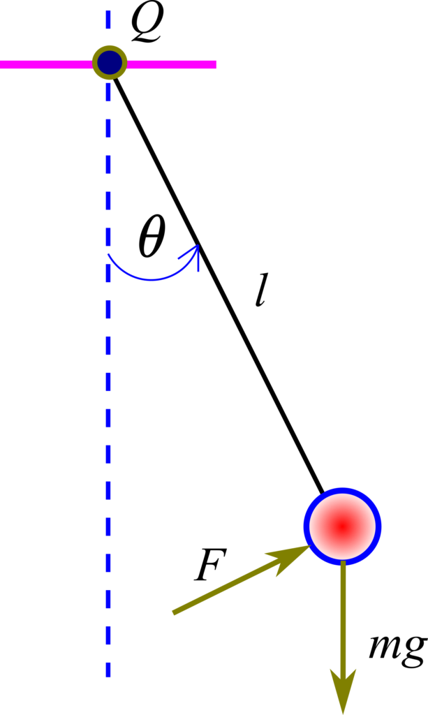
In our previous tutorial, which can be found here, we derived an equation of motion of this system. The equation of motion is given below

(1) $\begin{align*}\ddot{\theta}+\frac{g}{l}sin(\theta)=F\end{align*}$

where $g$ is the gravitational acceleration constant, $m$ is the mass of the ball, $l$ is the length of the rod, and $F$ is the external force acting on the ball. This force $F$ is perpendicular to the rod. Here, we assume that the force $F$ is a control force. Consequently, we can express this force as follows

(2) $\begin{align*}F=k\cdot u\end{align*}$

where $k$ is a constant and $u$ is the control input. From the previous two equations, we have

(3) $\begin{align*}\ddot{\theta}+\frac{g}{l}sin(\theta)=k\cdot u\end{align*}$

We rewrite this equation as follows

(4) $\begin{align*}\ddot{\theta}=- \frac{g}{l}sin(\theta) + k\cdot u \end{align*}$

Next, we introduce the state-space variables

(5) $\begin{align*}x_{1}=\theta \\x_{2}=\dot{\theta} \end{align*}$

In our previous tutorial, we explained how to derive the state space model. The state-space model has the following form

(6) $\begin{align*}\begin{bmatrix} \dot{x}_{1} \\ \dot{x}_{2} \end{bmatrix}=\begin{bmatrix} x_{2} \\ - \frac{g}{l}\sin(x_{1})+ku\end{bmatrix}\end{align*}$

This is a nonlinear state-space model because of the term $\sin(x_{1})$ . This term significantly complicates the control system design. If we would be able somehow to cancel this term, then we would significantly simplify the control system design.

In a nutshell, the main idea of feedback linearization is to determine a control input $u$ that will

Cancel the nonlinear term

(7) $\begin{align*}\frac{g}{l}\sin(x_{1}) \end{align*}$

on the right-hand side of the equation (6).

2. Assign (place) the poles of the feedback-linearized closed-loop system to desired locations such that the system is stabilized around the desired point.

In our case, we are interested in asymptotic stabilization of the control system around the stable equilibrium point $x_{1}=\theta=0$ . Of course, the feedback linearization approach can easily be generalized for the case of set-point tracking. That is, we can select any point around which we want to stabilize the system. This will be explained in future tutorials. For the time being, in order not to blur the main ideas of feedback linearization with too many details, we focus on the simplest possible case. That is, we focus on stabilization around the equilibrium point $x_{1}=\theta=0$ .

Here is the main idea of feedback linearization. We want the right-hand side of the second state-equation to be

(8) $\begin{align*} - \frac{g}{l}\sin(x_{1})+ku=-c_{0}x_{1}-c_{1}x_{2}\end{align*}$

where $c_{1}$ and $c_{2}$ are control parameters that we need to design such that the system is asymptotically stable. From the last equation, we obtain

(9) $\begin{align*}u=\frac{1}{k}\Big(\frac{g}{l}\sin(x_{1})-c_{0}x_{1}-c_{1}x_{2} \Big)\end{align*}$

The equation (9) is our feedback control law. Note that this is a state feedback control law that will “exactly” linearize the closed loop system. Although the closed-loop system will become linear, the feedback control law is still nonlinear. Let us substitute the control law (9) in our state-space model (6). As the result, we obtain

(10) $\begin{align*}\begin{bmatrix} \dot{x}_{1} \\ \dot{x}_{2} \end{bmatrix} & =\begin{bmatrix} x_{2} \\ - \frac{g}{l}\sin(x_{1})+k\cdot \frac{1}{k}\Big(\frac{g}{l}\sin(x_{1})-c_{0}x_{1}-c_{1}x_{2} \Big) \end{bmatrix} \\& =\begin{bmatrix} x_{2} \\ - \frac{g}{l}\sin(x_{1})+\frac{g}{l}\sin(x_{1})-c_{0}x_{1}-c_{1}x_{2} \end{bmatrix} \\& =\begin{bmatrix} x_{2} \\ -c_{0}x_{1}-c_{1}x_{2} \end{bmatrix}\end{align*}$

and consequently, we obtained a linear closed-loop system. That is, we have “exactly” linearized the nonlinear system.

The next task is to find the control system parameters $c_{0}$ and $c_{1}$ that will render the closed-loop system asymptotically stable. There are many ways to do that. Let us follow a textbook approach that is based on pole placement and computation of the characteristic polynomial.

The closed loop system can be written in the following form

(11) $\begin{align*}\begin{bmatrix} \dot{x}_{1} \\ \dot{x}_{2} \end{bmatrix} & =\begin{bmatrix}0 & 1 \\ -c_{0} & -c_{1} \end{bmatrix} \begin{bmatrix} x_{1} \\ x_{2} \end{bmatrix} \\\begin{bmatrix} \dot{x}_{1} \\ \dot{x}_{2} \end{bmatrix} & = A \begin{bmatrix} x_{1} \\ x_{2} \end{bmatrix}\end{align*}$

where the matrix $A$ is defined by

(12) $\begin{align*}A=\begin{bmatrix}0 & 1 \\ -c_{0} & -c_{1} \end{bmatrix} \end{align*}$

The characteristic polynomial is given as

(13) $\begin{align*}q(s)=\text{det}\big(sI - A \big)\end{align*}$

where

(14) $\begin{align*}sI - A =\begin{bmatrix} s & 0 \\ 0 & s \end{bmatrix}- \begin{bmatrix} 0 & 1 \\ -c_{0} & -c_{1} \end{bmatrix} =\begin{bmatrix} s & -1 \\ c_{0} & s+c_{1}\end{bmatrix}\end{align*}$

Consequently, the characteristic polynomial is

(15) $\begin{align*}q(s)=s(s+c_{1})+c_{0}=s^{2}+c_{1}s+c_{0}\end{align*}$

Let us place the closed-loop poles at the following locations

(16) $\begin{align*}s_{1}=-2,\;\; s_{2}=-4\end{align*}$

Consequently, the desired closed-loop characteristic polynomial is

(17) $\begin{align*}q_{\text{des}}=(s-s_{1})(s-s_{2})=(s+2)(s+4)=s^{2}+6s+8\end{align*}$

The desired polynomial should be equal to the parametrized characterized polynomial. That is, the equation (15) and the equation (17) should be equal. Consequently, we have

(18) $\begin{align*}& q_{\text{des}}=q(s) \\& s^{2}+6s+8=s^{2}+c_{1}s+c_{0}\end{align*}$

From this equation, we obtain the parameters $c_{0}$ and $c_{1}$ :

(19) $\begin{align*}c_{0}=8,\;\; c_{1}=6\end{align*}$

Next, we explain how to simulate the system in Simulink. First, we simulate the system without any control. That is we simulate the equation:

(20) $\begin{align*}\ddot{\theta}=-\frac{g}{l}\sin(\theta)\end{align*}$

The parameters for the simulation are

(21) $\begin{align*}g=9.81,\;\; l=1\end{align*}$

with the initial conditions

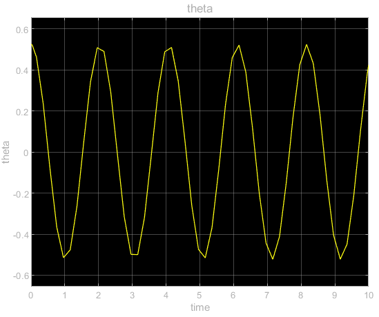
(22) $\begin{align*}\theta_{0}=\pi/6,\;\; \dot{\theta}_{0}=0\end{align*}$

The Simulink block diagram is given in the figure below.

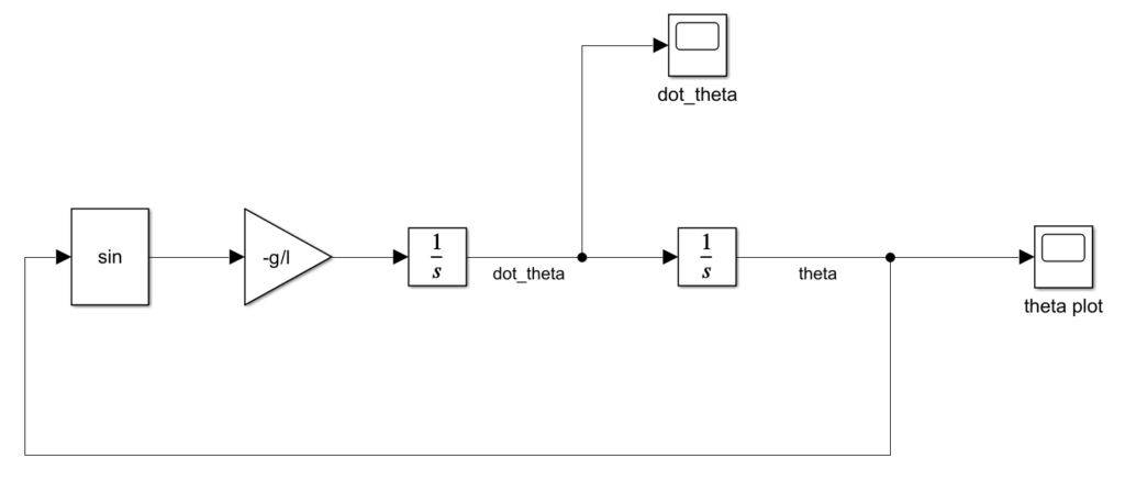
Figure: Simulink block diagram of the equation (20).

This block diagram solves the differential equation. The solution is shown in the figure below.

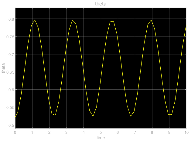
Next, we add a control input, and simulate the scaled step response. The equation we simulate is given below.

(23) $\begin{align*}\ddot{\theta}=-\frac{g}{l}\sin(\theta)+k\cdot u\end{align*}$

where we assume that

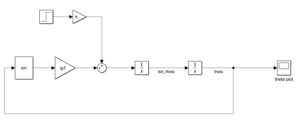
(24) $\begin{align*}g=9.81,\;\; l=1,\;\; \theta_{0}=\pi/6,\;\; \dot{\theta}_{0}=0,\;\; u=6\end{align*}$

The simulation results are given below.

Next, we simulate the feedback linearization control law. The control parameters (19) produce the following control law

(25) $\begin{align*}u& =\frac{1}{k}\Big(\frac{g}{l}\sin(x_{1})-8x_{1}-6x_{2} \Big) \\u& =\frac{1}{k}\Big(\frac{g}{l}\sin(\theta )-8\theta-6\dot{\theta} \Big)\end{align*}$

The block diagram corresponding to this control law is given below.

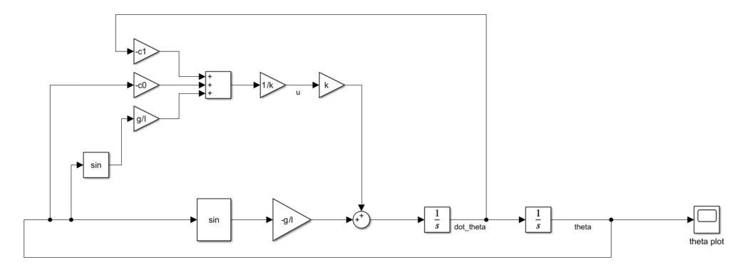
The response of the system is given below (theta variable).

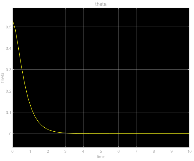
As we can observe, the system is asymptotically stabilized. That is, the closed-loop system is asymptotically stabilized by the feedback nonlinear control law.

admin

You might also like

Tutorial on Vector Containers in C++ Standard Template Library (STL)

Homework 1 – Strength of Materials – System That Cannot be in Static Equilibrium

Backward Euler Discretization of State-Space Models in MATLAB