Simulation of Ordinary Differential Equations (ODEs) with Time-varying Coefficients and Time-varying Inputs in MATLAB – Fusion of Engineering, Control, Coding, Machine Learning, and Science

In this post, we explain how to simulate Ordinary Differential Equations (ODEs) with time-varying coefficients and time-varying inputs in MATLAB.

Consider an ODE, given by the following equation

(1) $\begin{align*}\ddot{x}+k_{1}\dot{x}+k_{2}x=bu(t)\end{align*}$

where $k_{1}$ , $k_{2}$ , and $b$ are constants, and $u(t)$ is an external input that is a function of time. The goal is to simulate the solution of the ODE for an arbitrary time function $u(t)$ . In this particular example, we assumed that the constants $k_{1}$ , $k_{2}$ , and $b$ are constant. The presented approach can easily be generalized for ODEs with time varying constants $k_{1}$ , $k_{2}$ , and $b$ .

The first step is to write (1) in a state-space form. First, we introduce state-space variables

(2) $\begin{align*}x_{1}=x,\;\;\; x_{2}=\dot{x}\end{align*}$

Using these state-space variables, we can define a state-space model

(3) $\begin{align*}\underbrace{\begin{bmatrix} \dot{x}_{1} \\ \dot{x}_{2} \end{bmatrix}}_{\dot{\mathbf{x}}}= \underbrace{\begin{bmatrix} 0 & 1 \\ -k_{2} & -k_{1} \end{bmatrix}}_{A}\underbrace{\begin{bmatrix} x_{1} \\ x_{2} \end{bmatrix}}_{\mathbf{x}} +\underbrace{\begin{bmatrix} 0 \\ b \end{bmatrix}}_{B}u(t) \end{align*}$

Once we have formulated the state-space model, we can write a MATLAB code for simulating the ODE solution. Before we explain this code, we first have to explain the code for interpolating function values. The code and the post for interpolating function values are given here.

First, we define the state-space model matrices for arbitrary values of the parameters.

% test of ode45 integration with time varying inputs
% state-space model 
clear,clc,pack

% define the state-space matrices
A=[0 1; -0.1 -5], B=[0; 2], C=[1 0], D=[0]

Next, we define the time vector, input signal $u(t)$ , and an initial condition. We assume a sinusoidal input signal. The code is given below

time=0:0.1:100
input=sin(time)
x0=[2;1]

In order to simulate the dynamics, we need to define a MATLAB function whose value is the right-hand side of the equation (3). The function is given below.

function dxdt = dynamics(t, x, u, time_u,A,B)
input_int = interp1(time_u, u, t); % Interpolate the data set (time_u, u) at times t
dxdt = A*x+B*input_int; % Evalute ODE at times t

The first and second arguments of this function are the current time “t” and the current value of state “x”. The third argument is the input vector “u”. The fourth argument is the time vector. The entries of this time vector are used to define the input vector “u”. The last two parameters are the state-space matrices “A” and “B”. Code line 2 is used to compute the value of the input vector at the current time “t” (the current time “t” is the second argument of the function). This value is interpolated from the input function values that are defined by the vectors “u” and “time_u”. This interpolation approach also allows us to simulate the dynamics using a denser grid of points than the ones used to define the vectors “u” and “time_u”. Finally, code line 3 is used to evaluate the right-hand side of the equation (3) for the current value of state “x” and for the current value of input “u” that is defined by the interpolation scalar “input_int”. It is important to save this function in a separate file, whose name should be “dynamics.m”. Furthermore, the folder in which the file “dynamics.m” is stored should be included in MATLAB’s path. This is necessary because we plan to call this function from another MATLAB file (script).

The following code line is used to simulate the ODE dynamics

[time1 state_trajectory1] = ode45(@(t,x) dynamics(t, x, input, time,A,B), time, x0);

We use the built-in MATLAB function “ode45()”. The first argument is the name of the external function that is used to evaluate the right-hand side of the equation (3). The symbol “@(t,x)” in front of the function name is used to denote that “t” and “x” are the names of the time and state variables that are used to evaluate the right-hand side of the equation (3). The second argument of ode45 is the time vector at which we want to compute the solution, and the third argument is the initial state.

In order to test the validity of our approach, we compare it with another method for solving ODEs in MATLAB. Namely, we will use the Control Systems Toolbox and the function “lsim()” to simulate the state-space model. This is achieved by executing the following code lines.

sys=ss(A,B,C,D)
[output,time2,state_trajectory2] = lsim(sys,input,time,x0)

The function $ss()$ is used to define a state-space model, with the arguments “A”,”B”, “C”, and “D”. The state-space matrices $C$ and $D$ are used to define an output equation that is not relevant for our computations. The function “lsim()” us used to simulate the state-space model “sys”. We specify the input vector, as well as the time vector and the initial state. Next, we compute the error between the state trajectories computed using the two approaches, and we plot the state time series, as well as the error time series. The results are given in Fig. 1 and Fig. 2 below the code.

error = state_trajectory1(:,1)-state_trajectory2(:,1)

figure(1)
plot(time1,state_trajectory1(:,1),'r','LineWidth',6)
hold on
plot(time2,state_trajectory2(:,1),'k','LineWidth',2)

figure(2)
plot(error)

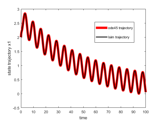
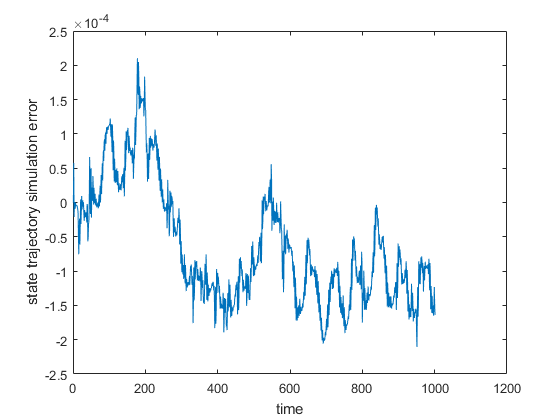
Figure 1: State time-series computed using the “ode45()” and “lsim()” MATLAB functions.

Figure 2: Error between the state trajectories computed using *the “ode45()” and “lsim()” MATLAB functions.*

By analyzing Fig. 1. and Fig. 2., we conclude that the two methods for solving ODEs produce almost identical results. The error is small and the state time series overlap.

admin

You might also like

Math/Control Systems Tutorial – Partial Fraction Expansion with MATLAB

Introduction to MATLAB System Identification Toolbox – Transfer Function Identification

The Factor of Safety and Simple Design Problems