 by
by
In this post, we provide a friendly introduction to MATLAB System Identification Toolbox. First, we define the system that we want to estimate and some system identification parameters.
The YouTube video accompanying this post is given below.
clear, pack, clc
zeta=0.4
wn=5

sampleTime=0.01
totalTime=5

system=tf([wn^2],[1 2*zeta*wn wn^2])
The transfer function has the following form
(1) 
where  is the damping ratio and
  is the undamped natural frequency.
The system identification problem is to estimate the transfer function parameters (coeffcients in the numerator and denumerator) from the collected input-output data.
In this tutorial, we perform the system identification experiments on the basis of the system’s step response. However, in practice, it is more desirable to use white noise or a sufficiently random signal to perform the system identification experiment instead of using a step signal. However, for the illustration purpose, we will use the step signal as an input and the corresponding step response as an output. Consequently, we first generate the identification data.
timeVector=[0:sampleTime:totalTime]';
initialState=[0;0];
input_step=ones(size(timeVector));
[simulatedOutputStep, timeVectorSimulatedStep]=lsim(system,input_step,timeVector,initialState);
figure(1)
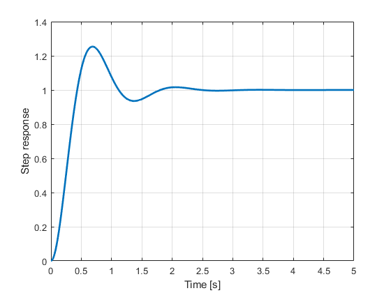
p1=plot(timeVectorSimulatedStep,simulatedOutputStep);
xlabel('Time [s]')
ylabel('Step response')
p1.LineWidth = 2
grid
The step response is shown in the figure below.
We need to create a data structure in order to estimate the system’s model. The function iddata() is used to formulate the data structure. The function arguments are system’s outputs and inputs.
%% perform system identification by using the step response to test the basic accuracy

% first, we test the results when the input is a step signal
% prepare the system identification data
systemIdentificationDataStep = iddata(simulatedOutputStep,input_step,sampleTime)
In this post, we will not cover the topic of estimating the model order. Consequently, we will use the exact model orders. In practice, when there is no a priori information about a good model order, the model order needs to be estimated from the data. The function used to estimate the model is tfest() . This function uses as inputs the data structure, number of poles of the estimated transfer function, and the number of zeros of the estimated transfer function.
% select the number of poles and zeros
np=2
nz=0
estimatedSystemStep = tfest(systemIdentificationDataStep,np,nz)

% Get list of model parameters and their uncertainties
[pvecStep, dpvecStep] = getpvec(estimatedSystemStep,'free')
covStep = getcov(estimatedSystemStep,'value','free')
The output of the function tfest() is:
estimatedSystemStep =

  From input "u1" to output "y1":
        25
  --------------
  s^2 + 4 s + 25

Continuous-time identified transfer function.

Parameterization:
   Number of poles: 2   Number of zeros: 0
   Number of free coefficients: 3
   Use "tfdata", "getpvec", "getcov" for parameters and their uncertainties.

Status:
Estimated using TFEST on time domain data "systemIdentificationDataStep".
Fit to estimation data: 100%
FPE: 2.626e-32, MSE: 2.574e-32
We can observe that we have obtained a perfect fit of the transfer function with almost zero estimation error. This is expected since the data is not corrupted by noise, the model to be estimated has the same structure of the data generated model, and we have assumed the correct model order (number of poles) and number of zeros.
Once we have estimated the model, we have used the functions getpvec() and getcov() to obtain uncertainties and covariances of the estimated parameters.
In reality, the measurement noise is always present. Consequently, we test the performance of the system identification function when the simulation (output) data is corrupted by noise. We take the simulated output data and we corrupt it by the measurement noise
% test the step response results with noise
simulatedOutputStepNoise = simulatedOutputStep+0.02*randn(size(simulatedOutputStep))

figure(2)
p2=plot(timeVectorSimulatedStep,simulatedOutputStepNoise)
xlabel('Time [s]')
ylabel('Noise-corrupted step response')
p2.LineWidth = 2
grid
The results are shown in the figure below.
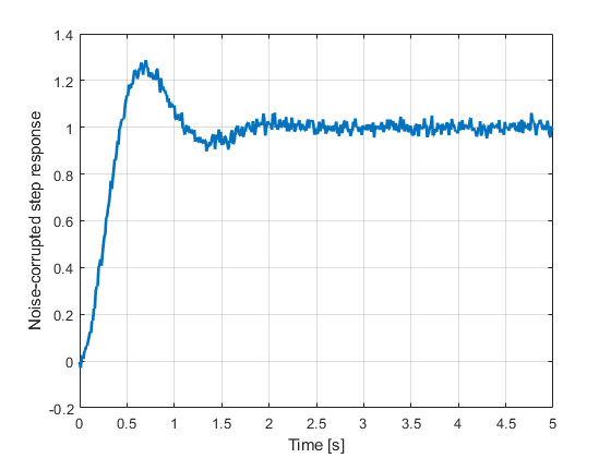
As we can see, the system identification data is quite noisy. We perform the system identification experiment.
systemIdentificationDataStepNoise = iddata(simulatedOutputStepNoise,input_step,sampleTime)
estimatedSystemStepNoise = tfest(systemIdentificationDataStepNoise,np,nz)

% Get list of model parameters and their uncertainties
[pvecStepNoise, dpvectNoise] = getpvec(estimatedSystemStepNoise,'free')
covStepNoise = getcov(estimatedSystemStepNoise,'value','free')
The estimation function produces the following results
estimatedSystemStepNoise =

  From input "u1" to output "y1":
          24.89
  ---------------------
  s^2 + 4.012 s + 24.88

Continuous-time identified transfer function.

Parameterization:
   Number of poles: 2   Number of zeros: 0
   Number of free coefficients: 3
   Use "tfdata", "getpvec", "getcov" for parameters and their uncertainties.

Status:
Estimated using TFEST on time domain data "systemIdentificationDataStepNoise".
Fit to estimation data: 90.52%
FPE: 0.0003797, MSE: 0.0003722
We can see the effect of the noise. Clearly, the noise affects the transfer function estimate. The next step is to simulate this model and compare the results with the data used for system identification. This is performed by the following code lines
% simulate the estimated model and compare it with the noisy data
[simulatedOutputStepEstimated, timeVectorSimulatedStepEstimated]=lsim(estimatedSystemStepNoise,input_step,timeVector,initialState);

figure(3)
p3=plot(timeVectorSimulatedStep,simulatedOutputStepNoise,timeVectorSimulatedStep,simulatedOutputStepEstimated)
xlabel('Time [s]')
ylabel('Noise-corrupted step response')
p3(1).LineWidth=2
p3(2).LineWidth=2
legend('Noisy step response','Estimated step response')
The results are shown in the figure below.
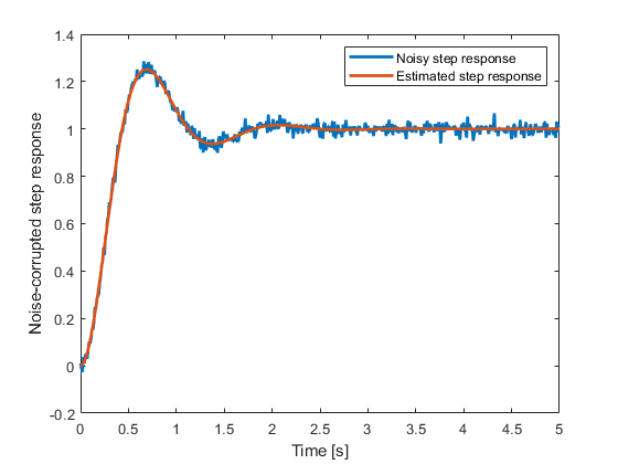
Another check of the model quality is to compare the estimated model (obtained from the noisy data) with the output of the noise-free model. By comparing the results you will observe that the outputs are almost identical.