Clear Explanation of the Ziegler-Nichols PID Control Tuning Method (Second Method) with MATLAB codes + Model Assisted Tuning – Fusion of Engineering, Control, Coding, Machine Learning, and Science

In this control engineering tutorial, we

Briefly explain the Ziegler-Nichols PID control tuning method. More precisely, we explain the second method based on increasing the proportional gain until stable and persistent oscillations occur in the response.
Explain how the model of the open-loop system can be combined with the Ziegler-Nichols method to quickly design preliminary PID control parameters.

The YouTube video accompanying this post is given below.

Summary of the Ziegler-Nichols PID Control Tuning Method (Second Method) with Example

The goal is to experimentally determine the parameters of the PID controller:

(1) $\begin{align*}C(s)=K_{p} \Big(1+\frac{1}{T_{i}s}+T_{d}s \Big)\end{align*}$

where $K_{p}$ is the proportional gain, $T_{i}$ is the parameter of the integral action, and $T_{d}$ is the parameter of the proportional action.

The first step is to set $T_{d}=0$ and to set $T_{i}=\infty$ (in practice, this is a very large value). That is, we only leave the proportional action. In that case, the controller is

(2) $\begin{align*}C(s)=K_{p}\end{align*}$

Let the plant be denoted by $P$ . Then, we have the following block diagram of the closed-loop system

Figure 1: Closed-loop system with the proportional gain $K_{p}$ .

where $r$ is the reference input (signal) and $y$ is the output of the closed-loop system.

Assuming that the applied reference input $r$ is an impulse (in practice, this can be a short pulse), our goal is to find the gain $K_{p}$ that produces stable and persistent oscillations of the output signal $y$ . Starting from zero, we keep on increasing $K_{p}$ until stable oscillation is observed. We read the period $L$ of such a stable oscillation. The period $L$ of stable oscillations is called the critical period or the ultimate period. The period $L$ is the input parameter for designing the PID controller. Let $K_{p}^{*}$ be the proportional gain that produces the stable oscillation. The proportional gain $K_{p}^{*}$ that produces the stable oscillation is called the critical gain or the ultimate gain.

The Ziegler-Nichols method determines the parameters of the PID controller as follows

(3) $\begin{align*}K_{p}=0.6 K_{p}^{*}, \;\; T_{i}=0.5 L,\;\; T_{d}=0.125 L\end{align*}$

On the other hand, if the controller is the PI controller, then the parameters are

(4) $\begin{align*}K_{p}=0.45 K_{p}^{*},\;\; T_{i}=\frac{1}{1.2} L\end{align*}$

Let us now illustrate the tuning method. To illustrate the tuning method, we assume that the plant is exactly

(5) $\begin{align*}P(s)=\frac{1}{s(s+2)(s+3)}\end{align*}$

This model is used to simulate the response (to generate the output). However, during the tuning process, we assume that we do not know this plant model. We only use the measured output of this model to obtain the response data. Only on the basis of the observed response data, we perform the PID controller tuning.

We use MATLAB to simulate the response of such a system. MATLAB codes are given later in the text.

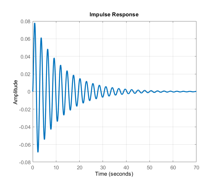
The (impulse) response of (5) for $K_{p}=5$ is given below.

We see that the impulse response “dies out” after some time. This is due to the fact that the closed-loop dynamics is asymptotically stable. The response for $K_{p}=25$ is given below.

The situation in Fig. 3 is little bit better. However, oscillations are still dying out. Finally, we show the response for $K_{p}=30$ .

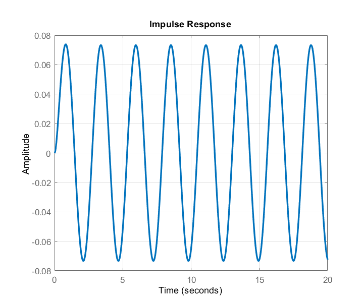We can see that for approximately $K_{p}=30$ , the impulse response becomes completely oscillatory and the oscillations are stable and persistent. On the other hand, if we increase the gain more, we will observe unable oscillations.

From this graph, we observe the period of the oscillation. The period of the oscillation $L$ is shown in the figure below.

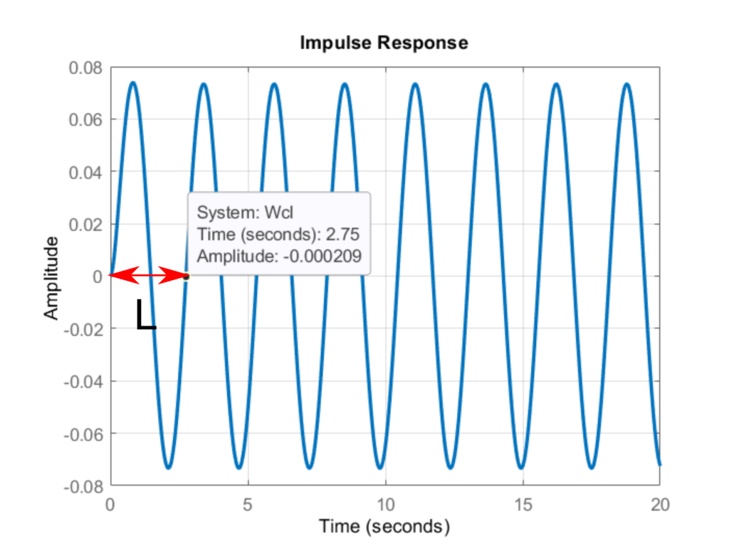Figure 5: Stable oscillations with the period $L$ .

We observe the period of oscillation of $L=2.75$ seconds. This is the main input parameter for designing the PID controller.

By using the Ziegler-Nichols method, we obtain the following parameters:

(6) $\begin{align*}K_{p}& =0.6\cdot 30 = 18 \\T_{i}& =0.5 \cdot 2.75 = 1.375 \\T_{d}& =0.125 \cdot 2.75 = 0.3438\end{align*}$

We can write the PID controller (1), as follows

(7) $\begin{align*}C(s)=\frac{K_{p}+K_{p}T_{i}s+K_{p}T_{d}T_{i}s^{2}}{T_{i}s}\end{align*}$

By substituting (6) in (7), we obtain

(8) $\begin{align*}C(s)=\frac{8.508 s^2 + 24.75 s + 18}{1.375 s}\end{align*}$

We simulate the step response of the closed loop system obtained by using (8). The results are shown in the figure below.

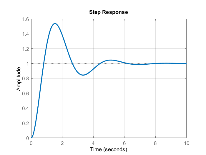
Figure 6: Step response of the closed-loop system.

We can observe that the closed-loop system has a zero steady-state error. However, it has a very large overshoot. We can reduce the overshoot by fine-tuning of the PID controller. We can decrease the overshoot by increasing the derivative action. This will decrease the overshoot, and at the same time decrease the speed of the response. To increase the speed of the response we increase the integral gain. The new coefficients are

(9) $\begin{align*}T_{d}^{new}& =2.5T_{d} \\T_{i}^{new}&=0.6T_{i} \\K_{p}^{new}&=K_{p}^{new}\end{align*}$

The modified controller is

(10) $\begin{align*}C^{new}(s)=\frac{12.76 s^2 + 14.85 s + 18}{0.825 s}\end{align*}$

The figure below compares the closed loop response of the original PID controller (Ziegler-Nichols PID controller) with the modified PID controller (Refined PID controller).

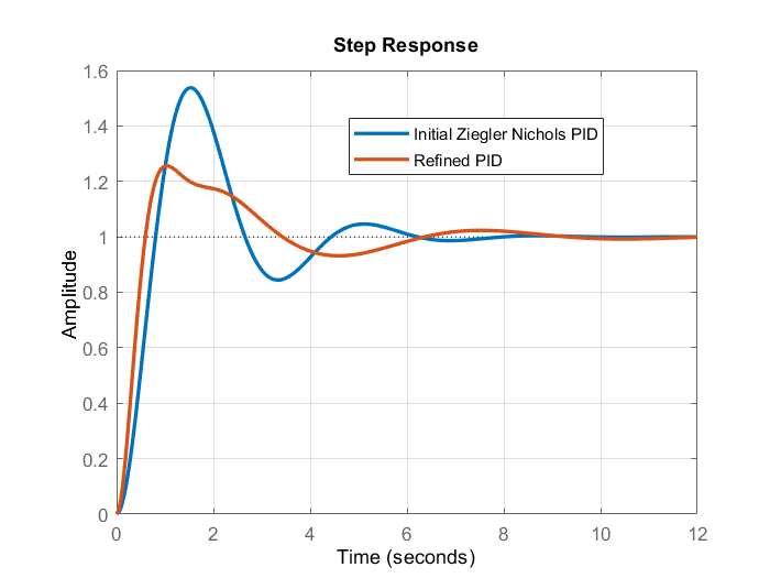
Figure 7: Closed-loop step response of the initial and refined PID controllers.

From Fig. 7, we can observe that the overshoot is decreased and that the rise time is improved compared to the initial Ziegler-Nichols PID controller. The MATLAB codes used to generate the graphs are given below.

% open-loop plant
% specify zeros, poles, and gain
close all, clear, clc
zeros=[]
poles=[0,-2,-3]
gain=1
P=zpk(zeros,poles,gain)

% proportional controller
propController=30

% create a closed-loop system
Wcl=feedback(propController*P,1)

% compute an impulse response
figure(1)
impulse(Wcl)

% computed parameters 
Kp=0.6*30
Ti=0.5*2.75
Td=0.125*2.75
C_PID=tf([Kp*Td*Ti Kp*Ti Kp],[Ti 0])
zpk(C_PID)
bode(C_PID)
% create a closed-loop system
Wcl2=feedback(C_PID*P,1)
figure(2)
hold on
step(Wcl2)

% increase the integral gain
% increase the derivative gain 

Ti2=0.6*Ti
Td2=2.5*Td

C_PID2=tf([Kp*Td2*Ti2 Kp*Ti2 Kp],[Ti2 0])
zpk(C_PID2)
Wcl3=feedback(C_PID2*P,1)
step(Wcl3)

Model-assisted Ziegler-Nichols PID Controller Tuning

Let us now explain how we can speed up the Ziegler-Nichols PID Controller Tuning if we have the model of the system. Let us assume that the model of the system (plant model) given by Eq. (5) is known. Here, for clarity, we rewrite the model.

(11) $\begin{align*}P(s)=\frac{1}{s(s+2)(s+3)}\end{align*}$

In the sequel, we explain how to determine the critical period $L$ and the critical gain $K_{p}^{*}$ without using the experimental data, that is, by only using the model of the system. In this way, we can decrease the experimental time duration, and obtain sufficiently accurate estimate of the critical gain $K_{p}^{*}$ . We can then test this gain and see if this gain produces the stable oscillations. If it does not, this means that our model is not accurate. However, even if the model is not accurate, the computed value of $K_{p}^{*}$ that is based on the inaccurate model can be a starting point for searching more appropriate value of the critical gain.

Let us assume that the controller is

(12) $\begin{align*}C(s)=K_{p}\end{align*}$

Then, the closed-loop characteristic polynomial is determined by the zeros of

(13) $\begin{align*}1+C(s)P(s)=1+\frac{K_{p}}{s(s+2)(s+3)}=0\end{align*}$

From this equation, we have

(14) $\begin{align*}s(s+2)(s+3)+K_{p}=0\end{align*}$

This polynomial can be written as follows

(15) $\begin{align*}s^3+5s^2+6s+K_{p}=0\end{align*}$

Self-sustained oscillations occur when the zeros (poles of the transfer function) of the characteristic polynomial are purely imaginary. That is, the zeros have the following form $s=j\omega$ , where $\omega$ is the angular frequency. By substituting $s=j\omega$ in (15), we obtain

(16) $\begin{align*}-j\omega^{3}-5\omega^2+6j\omega+K_{p}=0\end{align*}$

The complex polynomial is equal to zero when both its real and imaginary parts are zero. By using this fact, from (16), we see that the following two equations need to be satisfied (one for the real part and another for the imaginary part)

(17) $\begin{align*}K_{p}-5\omega^{2}=0\\-\omega^{3}+6\omega=0\end{align*}$

Since $\omega$ cannot be the solution, from the second equation, we obtain

(18) $\begin{align*}6-\omega^{2}=0,\;\; \omega=\sqrt{6}\end{align*}$

On the other hand, we have

(19) $\begin{align*}\omega=\frac{2\pi}{L}\end{align*}$

where $L$ is the previously introduced critical period. By substituting (18) in (19), we obtain

(20) $\begin{align*}\frac{2\pi}{L}=\sqrt{6}\\L=\frac{2\pi}{\sqrt{6}}=2.5651\end{align*}$

This value is very close to the value of $L=2.75$ that we found from Fig. 5. On the other hand, from the first equation in (17) and from (18), we find that

(21) $\begin{align*}K_{p}=5\omega^{2}=5\cdot 6=30\end{align*}$

and that is precisely the value of the critical gain that we have experimentally determined! Since we have determined the critical period and the critical gain from the plant model, from here, we can use the Ziegler-Nichols equations (6) to design the parameters of the PID controller.

To summarize, we learned how to use the model of the plant to quickly determine the critical period and the critical gain that can be used to design the Ziegler Nichols PID controller.

Summary of the Ziegler-Nichols PID Control Tuning Method (Second Method) with Example

Model-assisted Ziegler-Nichols PID Controller Tuning

admin

You might also like

Install MicroBlaze Processor and Start with C/C++ Coding FPGAs in Vivado and Vitis

How to Reverse Animations in Blender

Test 4