Introduction to inverse kinematics of robots – Fusion of Engineering, Control, Coding, Machine Learning, and Science

In this post, we explain how to solve an inverse kinematics problem of a robot with two degrees of freedom. In this relatively simple case, it is possible to solve the inverse kinematics problem analytically (that is, to compute the closed-form solution). The purpose of this example is to introduce the inverse kinematics problem. The YouTube video accompanying this post can be found here

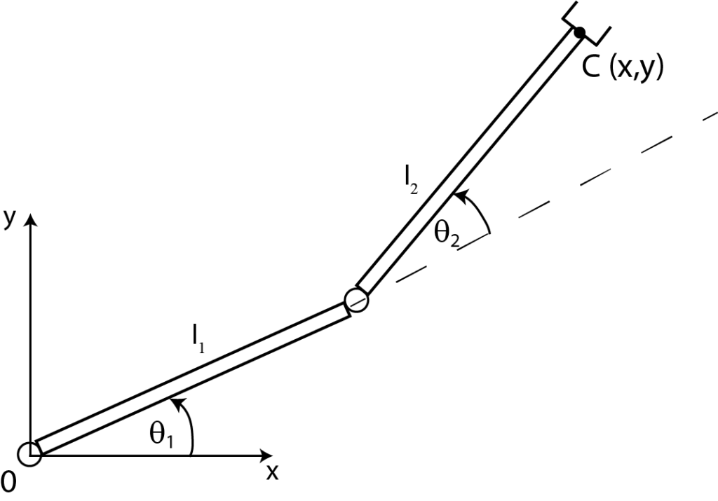
Consider a manipulator with two rotational degrees of freedom $\theta_{1}$ and $\theta_{2}$ shown in the figure below.

Figure 1: two degrees of freedom robotic manipulator for explaining the inverse kinematics problem.

The inverse kinematics problem can be formulated as follows:

Given the coordinates x and y of the end-effector point C (world coordinates), compute the angles $\theta_{1}$ and $\theta_{2}$ (local joint coordinates).

In the statement of the inverse kinematics problem, it is assumed that the lengths of the robotic segments $l_{1}$ and $l_{2}$ are given.

From Figure 1, we have

(1) $\begin{align*}x=l_{1}cos(\theta_{1})+l_{2}cos(\theta_{1}+\theta_{2}) \\y=l_{1}sin(\theta_{1})+l_{2}sin(\theta_{1}+\theta_{2})\end{align*}$

By squaring the last two equations and adding them together, we obtain

(2) $\begin{align*}&x^{2}+y^{2}=l_{1}^{2}+l_{2}^{2}+2l_{1}l_{2}\Big(cos(\theta_{1})cos(\theta_{1}+\theta_{2})+sin(\theta_{1})sin(\theta_{1}+\theta_{2}) \Big) \end{align*}$

Next, we use the following trigonometric formula

(3) $\begin{align*}cos(a_{1}-a_{2})=cos(a_{1})cos(a_{2})+sin(a_{1})sin(a_{2})\end{align*}$

By using this formula with $a_{1}=\theta_{1}$ and $a_{2}=\theta_{2}$ , from (2), we have

(4) $\begin{align*}x^{2}+y^{2}=& l_{1}^{2}+l_{2}^{2}+2l_{1}l_{2}cos(-\theta_{2}) \\=& l_{1}^{2}+l_{2}^{2}+2l_{1}l_{2}cos(\theta_{2})\end{align*}$

where we have used the identity $cos(-\theta_{2})=cos(\theta_{2})$ (cosine function is an even function). From the last equation, we have

(5) $\begin{align*}cos(\theta_{2})=\frac{x^{2}+y^{2}-l_{1}^2-l_{2}^2}{2l_{1}l_{2}} \end{align*}$

The last equation enables us to compute the angle $\theta_{1}$ as a function of $x$ and $y$ .

Here, an important observation should be made. Let us assume that the right-hand of the equation (5) is equal to $0.5$ . To compute $\theta_{2}$ , we need to solve this equation

(6) $\begin{align*}cos(\theta_{2})=0.5\end{align*}$

This equation has an infinite number of solutions, however, there are only two solutions that are physically unique and physically realistic, these solutions are

(7) $\begin{align*}\theta_{2}=60,\;\;\theta_{2}=-60 \end{align*}$

The figure below illustrates a similar scenario. We can observe that there are two possibilities for reaching point C (red and black manipulator positions).

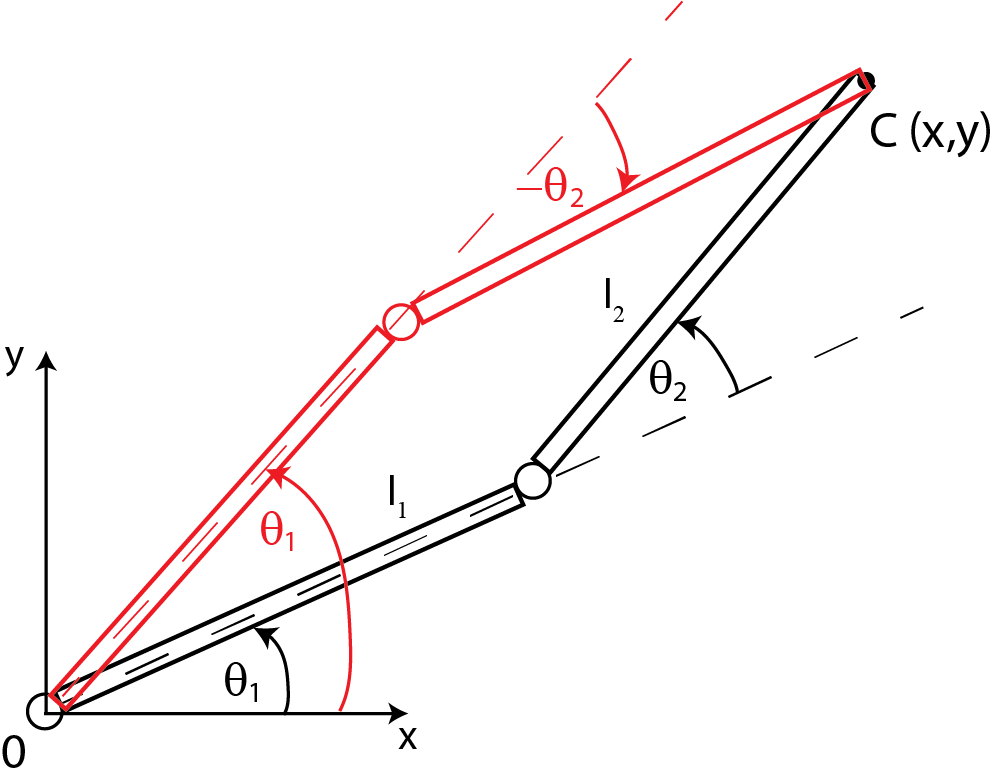
Figure 2: non-uniqueness of the inverse kinematics problem.

This is a common situation when solving the inverse kinematics problem.

We will determine the angle $\theta_{1}$ by analyzing the figure shown below.

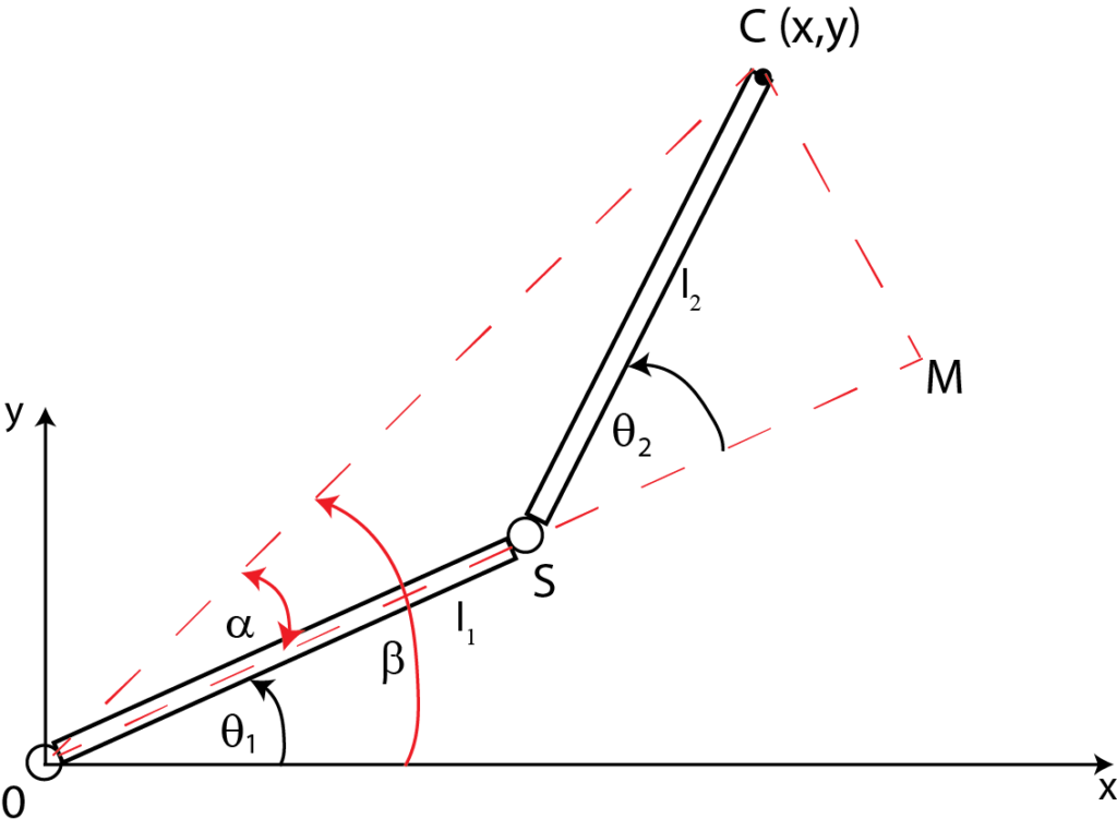Figure 3: Figure for determining $\theta_{1}$ .

From the figure 3, we have

(8) $\begin{align*}\theta_{1}=\beta - \alpha\end{align*}$

where $\beta$ and $\alpha$ are angles shown in the figure below. We will find $\theta_{1}$ by using the tan() function. From (8), we have

(9) $\begin{align*}\tan (\theta_{1})=\tan(\beta - \alpha)\end{align*}$

Next, we will use the following formula

(10) $\begin{align*}\tan (\theta_{1})=\tan(\beta - \alpha)= \frac{\tan(\beta)-\tan(\alpha)}{1+\tan(\beta)\tan(\alpha)}\end{align*}$

From Fig. 3, we have

(11) $\begin{align*}\tan(\beta)=\frac{y}{x}\end{align*}$

on the other hand, from triangles OMC and CMS, we have

(12) $\begin{align*}\tan(\alpha) = \frac{\overline{CM}}{\overline{OS}+\overline{SM}}=\frac{l_{2}\sin(\theta_{2})}{l_{1}+l_{2}\cos(\theta_{2})}\end{align*}$

Here, it should be noted that $\alpha$ is only a function of $\theta_{2}$ , so once $\theta_{2}$ is determined from (5), we can find $\alpha$ from (12).

By substituting (11) and (12) in (10), we obtain the final result for $\theta_{1}$

(13) $\begin{align*}\tan(\theta_{1}) = \frac{y(l_{1}+l_{2}\cos(\theta_{2}))-xl_{2}\sin(\theta_{2})}{x(l_{1}+l_{2}\cos(\theta_{2}))+y l_{2} \sin(\theta_{2})}\end{align*}$

admin

You might also like

Intro to Machine Learning 1: Using TensorFlow (Keras) to Solve a Quadratic Equation

3D surface plot of functions in MATLAB using the function fsurf()

Write Numerical or Text Data to File in C Programming Language