Intro to Machine Learning 1: Using TensorFlow (Keras) to Solve a Quadratic Equation – Fusion of Engineering, Control, Coding, Machine Learning, and Science

This post is the first post in a series of posts on the basic principles of machine learning and Phyton machine learning libraries.

In this post, we investigate the possibility of using a “brute force” machine learning approach to solve a quadratic equation. The video accompanying this post is given here:

(1) $\begin{align*}ax^{2}+bx+c=0\end{align*}$

where $a,b,c\in \mathbb{R}$ are constants and $x\in \mathbb{R}$ is unknown variable. The solution is given the quadratic formula

(2) $\begin{align*}x_{1,2}=\frac{-b \pm \sqrt{b^2-4ac}}{2a}\end{align*}$

Our probem can be stated as follows. For given constants $a,b$ and $c$ use neural networks to compute the solutions $x_{1}$ and $x_{2}$ without using the quadratic formula. So how can we find the solution without using the quadratic formula? Well, if we had a set of coefficients $C=\{ (a_{i},b_{i},c_{i}) | i=1,2,\ldots, N \}$ and the set of the corresponding solutions $S= \{ (x_{1}^{(i)}, x_{2}^{(i)} ) | i=1,2,\ldots, N \}$ , then we could try to “learn” a rule or mathematical model that maps S to C. In this post, our mathematical model is an artificial neural network (ANN):

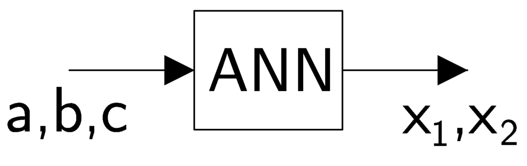
Using control theory and machine learning terminologies, we refer to the coefficients $a,b$ and $c$ as inputs, and the solutions $x_{1}$ and $x_{2}$ are referred to as outputs.

We use the Keras machine learning library to solve this problem. Keras is run on top of TensorFlow machine learning library. First, we import all the necessary libraries.

import numpy as np
import matplotlib.pyplot as plt
import cmath
import time
import tensorflow as tf
from keras import models
from keras import layers
from keras.optimizers import RMSprop
from keras.optimizers import Adam
from keras.callbacks import ModelCheckpoint

A few comments are in order. The lines 1-4 are used to import libraries handing matrices, plotting, complex numbers, and time measurements, respectively. The code line 5 is used to load the TensorFlow library. The code lines 6 and 7 are used to load Keras functions for defining models and layers, respectively. The code lines 8 and 9 are used to load the Keras optimizer and the code line 10 is used to load the function for saving models during the network training. This function enables us to save the model with the best validation performance and to do so, during every epoch (the notion of epochs will be defined later in the text). Next, we define the total number of multidimensional training, validation, and test data points, which is usually referred to as the sample number, and in our code it is denoted by “sample_number”:

sample_number=10000

The next step is to define the training data. As its name implies, the training data is the data used to optimize (or in layman’s terms “to train”) the model weights. The training data is defined as follows:

# training data
atrain=np.random.rand(sample_number,1)
btrain=np.random.rand(sample_number,1)
ctrain=np.random.rand(sample_number,1)

dataXtrain=np.concatenate((atrain,btrain,ctrain),axis=1)

x1real_train=np.zeros(shape=(sample_number,1))
x1imag_train=np.zeros(shape=(sample_number,1))
x2real_train=np.zeros(shape=(sample_number,1))
x2imag_train=np.zeros(shape=(sample_number,1))


for i in range(sample_number):
    x1=(-btrain[i,0]+cmath.sqrt(btrain[i,0]**2-4*atrain[i,0]*ctrain[i,0]))/(2*atrain[i,0])
    x2=(-btrain[i,0]-cmath.sqrt(btrain[i,0]**2-4*atrain[i,0]*ctrain[i,0]))/(2*atrain[i,0])
    x1real_train[i,0]=np.real(x1)
    x1imag_train[i,0]=np.imag(x1)
    x2real_train[i,0]=np.real(x2)
    x2imag_train[i,0]=np.imag(x2)

dataYtrain=np.concatenate((x1real_train,x1imag_train,x2real_train,x2imag_train),axis=1)

The code lines 2-4 are used to define the input parameters a,b, and c. Every coefficient is a random number drawn from a uniform distribution defined in the interval [0,1]. All the input parameters are defined as vectors and stacked column-wise to define the input matrix on the code line 6. Next, we proceed with the definition of the output data. The code lines 8-11 are used to reserve the memory space for real and imaginary parts of the solutions $x_{1}$ and $x_{2}$ . This might not be the most optimal and data saving approach for defining the output data (the question for the reader “Why?”), however, despite that we proceed with this approach for clarity and simplicity. The output vector are defined as follows:

for i in range(sample_number):
    x1=(-btrain[i,0]+cmath.sqrt(btrain[i,0]**2-4*atrain[i,0]*ctrain[i,0]))/(2*atrain[i,0])
    x2=(-btrain[i,0]-cmath.sqrt(btrain[i,0]**2-4*atrain[i,0]*ctrain[i,0]))/(2*atrain[i,0])
    x1real_train[i,0]=np.real(x1)
    x1imag_train[i,0]=np.imag(x1)
    x2real_train[i,0]=np.real(x2)
    x2imag_train[i,0]=np.imag(x2)

dataYtrain=np.concatenate((x1real_train,x1imag_train,x2real_train,x2imag_train),axis=1)

The for loop 1-7 is implementing the formula for the solution of quadratic equations. The code line 9 is used to define the output matrix. This matrix is defined by stacking the real and imaginary parts of the two solutions $x_{1}$ and $x_{2}$ . Next, using the same procedure, we define the validation and training data.

# validation data
aval=np.random.rand(sample_number,1)
bval=np.random.rand(sample_number,1)
cval=np.random.rand(sample_number,1)

dataXval=np.concatenate((aval,bval,cval),axis=1)

x1real_val=np.zeros(shape=(sample_number,1))
x1imag_val=np.zeros(shape=(sample_number,1))
x2real_val=np.zeros(shape=(sample_number,1))
x2imag_val=np.zeros(shape=(sample_number,1))


for i in range(sample_number):
    x1=(-bval[i,0]+cmath.sqrt(bval[i,0]**2-4*aval[i,0]*cval[i,0]))/(2*aval[i,0])
    x2=(-bval[i,0]-cmath.sqrt(bval[i,0]**2-4*aval[i,0]*cval[i,0]))/(2*aval[i,0])
    x1real_val[i,0]=np.real(x1)
    x1imag_val[i,0]=np.imag(x1)
    x2real_val[i,0]=np.real(x2)
    x2imag_val[i,0]=np.imag(x2)

dataYval=np.concatenate((x1real_val,x1imag_val,x2real_val,x2imag_val),axis=1)



# test data
atest=np.random.rand(sample_number,1)
btest=np.random.rand(sample_number,1)
ctest=np.random.rand(sample_number,1)

dataXtest=np.concatenate((atest,btest,ctest),axis=1)

x1real_test=np.zeros(shape=(sample_number,1))
x1imag_test=np.zeros(shape=(sample_number,1))
x2real_test=np.zeros(shape=(sample_number,1))
x2imag_test=np.zeros(shape=(sample_number,1))


for i in range(sample_number):
    x1=(-btest[i,0]+cmath.sqrt(btest[i,0]**2-4*atest[i,0]*ctest[i,0]))/(2*atest[i,0])
    x2=(-btest[i,0]-cmath.sqrt(btest[i,0]**2-4*atest[i,0]*ctest[i,0]))/(2*atest[i,0])
    x1real_test[i,0]=np.real(x1)
    x1imag_test[i,0]=np.imag(x1)
    x2real_test[i,0]=np.real(x2)
    x2imag_test[i,0]=np.imag(x2)

dataYtest=np.concatenate((x1real_test,x1imag_test,x2real_test,x2imag_test),axis=1)

The validation data is used during the training to validate the trained model on a new data set. The model with the best validation performance will be saved in a file. This model is referred to as the best model. The test data is used to test the performance of the best model. Next, we define the neural network model, set-up the solvers and parameters, and train the network. At the end of the code, we test the performance of the best model and plot the results.

###############################################################################
#                            network
###############################################################################
with tf.device('/cpu:0'): 
    network = models.Sequential()
    network.add(layers.Dense(5, activation='tanh',kernel_initializer='random_normal',use_bias=False,input_dim=3))
    network.add(layers.Dense(5, activation='tanh',kernel_initializer='random_normal', use_bias=False))
    network.add(layers.Dense(5, activation='tanh',kernel_initializer='random_normal', use_bias=False))
    #network.add(layers.Dense(20, activation='relu',kernel_initializer='random_uniform', use_bias=False))
    network.add(layers.Dense(4, activation = 'linear',kernel_initializer='random_normal',use_bias=False))
    network.compile(optimizer=RMSprop(), loss='mean_squared_error', metrics=['mse'])
    #network.compile(optimizer=RMSprop(), loss='mean_absolute_percentage_error', metrics=['mse'])  # 'mean_absolute_percentage_error' is another option
    #network.compile(optimizer=Adam(), loss='mean_squared_error')
    
    
    # only save the model with the best validation loss value
    filepath="\\python_codes\\quadratic_equation\\best_model.hdf5"
    checkpoint = ModelCheckpoint(filepath, monitor='val_loss', verbose=0, save_best_only=True, save_weights_only=False, mode='min')
    callbacks_list = [checkpoint]
    start_time = time.time()
    history=network.fit(dataXtrain,dataYtrain,epochs=100000, batch_size=2000,callbacks=callbacks_list, validation_data=(dataXval,dataYval), verbose=2)
    end_time = time.time()
    print('Training time %f'%(end_time-start_time))     
###############################################################################
#                    Plot the history    
###############################################################################
    
loss=history.history['loss']
val_loss=history.history['val_loss']
epochs=range(1,len(loss)+1)
plt.figure()
plt.plot(epochs, loss,'b', label='Training loss')
plt.plot(epochs, val_loss,'r', label='Validation loss')
plt.title('Training and validation losses')
plt.xlabel('Epochs')
plt.ylabel('Loss')
plt.xscale('log')
plt.yscale('log')
plt.legend()
plt.savefig('loss_curves4.png')
plt.show()

###############################################################################
#                   test the model prediction performance
###############################################################################
network.load_weights(filepath)

dataYtrain_prediction=network.predict(dataXtrain)
dataYval_prediction=network.predict(dataXval)
dataYtest_prediction=network.predict(dataXtest)


x1real_test[i,0]=np.real(x1)
x1imag_test[i,0]=np.imag(x1)
x2real_test[i,0]=np.real(x2)
x2imag_test[i,0]=np.imag(x2)

x1real_test_prediction=np.zeros(shape=(sample_number,1))
x1imag_test_prediction=np.zeros(shape=(sample_number,1))
x2real_test_prediction=np.zeros(shape=(sample_number,1))
x2imag_test_prediction=np.zeros(shape=(sample_number,1))

for i in range(sample_number):
    x1real_test_prediction[i,0]=dataYtest_prediction[i,0]
    x1imag_test_prediction[i,0]=dataYtest_prediction[i,1]
    x2real_test_prediction[i,0]=dataYtest_prediction[i,2]
    x2imag_test_prediction[i,0]=dataYtest_prediction[i,3]
    
plt.plot(x1real_test,x1imag_test,'bo',markersize=7,label='True solution')    
plt.plot(x2real_test,x2imag_test,'bo',markersize=7) 
plt.plot(x1real_test_prediction,x1imag_test_prediction,'rx',markersize=7,label='Predicted solution')    
plt.plot(x2real_test_prediction,x2imag_test_prediction,'rx',markersize=7)    
plt.xlabel('Real part')
plt.ylabel('Imaginary part')
plt.xlim(-100, 10)
plt.ylim(-15, 15)
plt.legend()
plt.savefig('identified4.png')
plt.show()

A few comments are in order. The code line 4 is used to force TensorFlow to run on a CPU. This line can be changed such that the code is run on a GPU. The code lines 5-10 are used to define the network model. The code line 5 is telling Keras that we are defining a sequential network (a network defined by stacking layers). The code line 6 is used to define the input layer. The input dimension, denoted by “input_dim=3″, is used to define the number of inputs (we have three inputs: a,b, and c). The code lines 7-9 are used to define the inner layers with an arbitrary number of neurons (which is the first parameter in the function ” layers.Dense()”). The code 10 is used to define the output layer. Notice that the output layer has 4 neurons since we have 4 outputs (real and imaginary parts of $x_{1}$ and x_{2}). The code line 11 is used to compile the network and to define the optimizer and its parameters. The code lines 17-19 are used to create a “model checkpoint”. In Keras terminology, the model checkpoint is used to save the model with the best validation loss. That is, during each training epoch, using the validation input data and the current trained model, we generate the predicted validation data. The validation loss is then computed on the basis of this predicted validation data and the validation data that is generated on the basis of the exact formula (this validation data is defined in the previous code snippet). If the trained model has a better validation loss than the previously saved model, then this model is saved (the model file is overwritten). The file path is defined by:

filepath=”\\python_codes\\quadratic_equation\\best_model.hdf5″

which corresponds to the path:
C:\python_codes\quadratic_equation\best_model.hdf5
on the disk C on my computer. You have to create the folder “C:\python_codes\quadratic_equation\ ” in order for this code to execute.

The code lines 20 and 22 are used to measure the time it takes for the training code to execute. The code line 21 is used to train the network. The “history” is a Python dictionary file used to save training and validation losses. The code lines 28-41 are used to save the plots of the training and validation curves. The code line 46 is used to load the best model. The code lines 48-79 are used to generate the predictions on the basis of the test data and to plot the results.

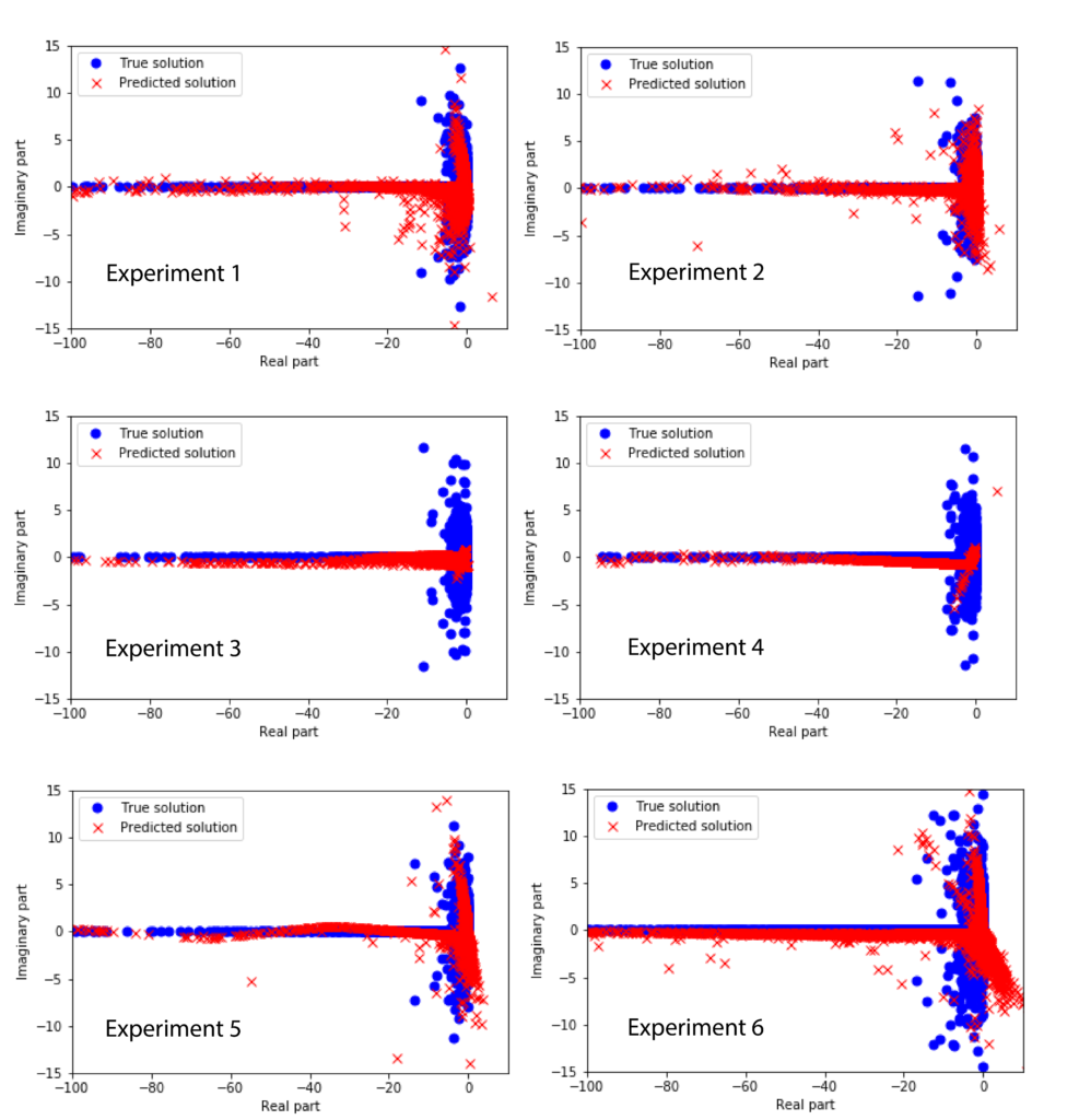
The following figure shows the exact and predicted solutions on the basis of the test data for different experimental conditions (see the explanation at the end of the post).

The following figure shows the training and validation curves for six performed experiments.

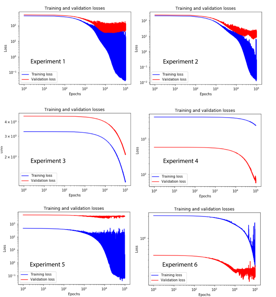
The experimental conditions differ in the number of layers, neurons, and samples. The experimental conditions are defined as follows.

Experiment 1:

sample_number=10000

    network = models.Sequential()
    network.add(layers.Dense(100, activation='tanh',kernel_initializer='random_normal',use_bias=False,input_dim=3))
    network.add(layers.Dense(100, activation='tanh',kernel_initializer='random_normal', use_bias=False))
    network.add(layers.Dense(100, activation='tanh',kernel_initializer='random_normal', use_bias=False))
    #network.add(layers.Dense(20, activation='relu',kernel_initializer='random_uniform', use_bias=False))
    network.add(layers.Dense(4, activation = 'linear',kernel_initializer='random_normal',use_bias=False))
    network.compile(optimizer=RMSprop(), loss='mean_squared_error', metrics=['mse'])
    #network.compile(optimizer=RMSprop(), loss='mean_absolute_percentage_error', metrics=['mse'])  # 'mean_absolute_percentage_error' is another option
    #network.compile(optimizer=Adam(), loss='mean_squared_error')

Experiment 2:

sample_number=10000

    network = models.Sequential()
    network.add(layers.Dense(50, activation='tanh',kernel_initializer='random_normal',use_bias=False,input_dim=3))
    network.add(layers.Dense(50, activation='tanh',kernel_initializer='random_normal', use_bias=False))
    network.add(layers.Dense(50, activation='tanh',kernel_initializer='random_normal', use_bias=False))
    #network.add(layers.Dense(20, activation='relu',kernel_initializer='random_uniform', use_bias=False))
    network.add(layers.Dense(4, activation = 'linear',kernel_initializer='random_normal',use_bias=False))
    network.compile(optimizer=RMSprop(), loss='mean_squared_error', metrics=['mse'])
    #network.compile(optimizer=RMSprop(), loss='mean_absolute_percentage_error', metrics=['mse'])  # 'mean_absolute_percentage_error' is another option
    #network.compile(optimizer=Adam(), loss='mean_squared_error')
    

Experiment 3:

sample_number=10000

###############################################################################
with tf.device('/gpu:0'): 
    network = models.Sequential()
    network.add(layers.Dense(10, activation='tanh',kernel_initializer='random_normal',use_bias=False,input_dim=3))
    network.add(layers.Dense(10, activation='tanh',kernel_initializer='random_normal', use_bias=False))
    network.add(layers.Dense(10, activation='tanh',kernel_initializer='random_normal', use_bias=False))
    #network.add(layers.Dense(20, activation='relu',kernel_initializer='random_uniform', use_bias=False))
    network.add(layers.Dense(4, activation = 'linear',kernel_initializer='random_normal',use_bias=False))
    network.compile(optimizer=RMSprop(), loss='mean_squared_error', metrics=['mse'])
    #network.compile(optimizer=RMSprop(), loss='mean_absolute_percentage_error', metrics=['mse'])  # 'mean_absolute_percentage_error' is another option
    #network.compile(optimizer=Adam(), loss='mean_squared_error')

Experiment 4:

sample_number=10000


with tf.device('/cpu:0'): 
    network = models.Sequential()
    network.add(layers.Dense(5, activation='tanh',kernel_initializer='random_normal',use_bias=False,input_dim=3))
    network.add(layers.Dense(5, activation='tanh',kernel_initializer='random_normal', use_bias=False))
    network.add(layers.Dense(5, activation='tanh',kernel_initializer='random_normal', use_bias=False))
    #network.add(layers.Dense(20, activation='relu',kernel_initializer='random_uniform', use_bias=False))
    network.add(layers.Dense(4, activation = 'linear',kernel_initializer='random_normal',use_bias=False))
    network.compile(optimizer=RMSprop(), loss='mean_squared_error', metrics=['mse'])
    #network.compile(optimizer=RMSprop(), loss='mean_absolute_percentage_error', metrics=['mse'])  # 'mean_absolute_percentage_error' is another option
    #network.compile(optimizer=Adam(), loss='mean_squared_error')



Experiment 5:


sample_number=10000

with tf.device('/cpu:0'): 
    network = models.Sequential()
    network.add(layers.Dense(200, activation='tanh',kernel_initializer='random_normal',use_bias=False,input_dim=3))
    network.add(layers.Dense(200, activation='tanh',kernel_initializer='random_normal', use_bias=False))
    network.add(layers.Dense(200, activation='tanh',kernel_initializer='random_normal', use_bias=False))
    network.add(layers.Dense(200, activation='tanh',kernel_initializer='random_normal', use_bias=False))
    network.add(layers.Dense(200, activation='tanh',kernel_initializer='random_normal', use_bias=False))
    #network.add(layers.Dense(20, activation='relu',kernel_initializer='random_uniform', use_bias=False))
    network.add(layers.Dense(4, activation = 'linear',kernel_initializer='random_normal',use_bias=False))
    network.compile(optimizer=RMSprop(), loss='mean_squared_error', metrics=['mse'])
    #network.compile(optimizer=RMSprop(), loss='mean_absolute_percentage_error', metrics=['mse'])  # 'mean_absolute_percentage_error' is another option
    #network.compile(optimizer=Adam(), loss='mean_squared_error')
    


Experiment 6:

sample_number=50000

###############################################################################
with tf.device('/cpu:0'): 
    network = models.Sequential()
    network.add(layers.Dense(100, activation='tanh',kernel_initializer='random_normal',use_bias=False,input_dim=3))
    network.add(layers.Dense(100, activation='tanh',kernel_initializer='random_normal', use_bias=False))
    network.add(layers.Dense(100, activation='tanh',kernel_initializer='random_normal', use_bias=False))
#    network.add(layers.Dense(200, activation='tanh',kernel_initializer='random_normal', use_bias=False))
#    network.add(layers.Dense(200, activation='tanh',kernel_initializer='random_normal', use_bias=False))
    #network.add(layers.Dense(20, activation='relu',kernel_initializer='random_uniform', use_bias=False))
    network.add(layers.Dense(4, activation = 'linear',kernel_initializer='random_normal',use_bias=False))
    network.compile(optimizer=RMSprop(), loss='mean_squared_error', metrics=['mse'])
    #network.compile(optimizer=RMSprop(), loss='mean_absolute_percentage_error', metrics=['mse'])  # 'mean_absolute_percentage_error' is another option
    #network.compile(optimizer=Adam(), loss='mean_squared_error')

Assignments. Improve the results by increasing the sample number or changing the network architecture. Also, you can change the activation functions.

admin

You might also like

Test 4

Blender Tutorial: Animate an Object Following a Predefined Trajectory

Setting up Raspberry Pi for Mechatronics Projects – 1