 by
by This post and the follow-up video explain how to detect (recognize) contours of an image in OpenCV (Python). If you are completely new to OpenCV, you can start with our previous post in which we explained how to load, resize, and save images by using OpenCV. The YouTube video accompanying this post is given below.
Contour detection is important for many fields. In the next post, we will explain how to use contour detection in order to build a computer vision system for pick and place robotics tasks.
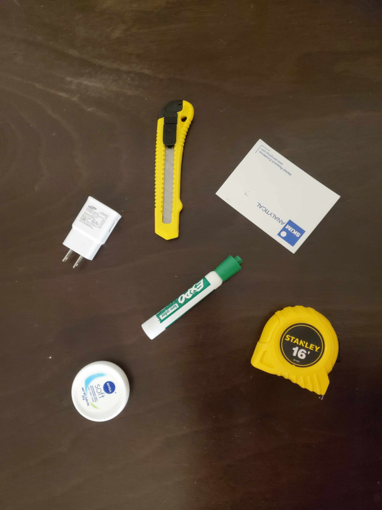
We use the image shown below to demonstrate contour detection. You can freely download this image and save it to your disk. To download this image, right-click on the image and then click on “Save image as”. Save the image as “partsTest.png”. Make sure that a Python script file is in the same folder as the saved image.
The result of the contour detection is given below.

The following code lines are used to load the image, resize the image, and save the resized image to disk.
import cv2
from matplotlib import pyplot as plt
import numpy as np

# keep in mind that open CV loads images as BGR not RGB
image = cv2.imread("partsTest.png")
cv2.imshow('Image',image)
cv2.waitKey(0)
cv2.destroyAllWindows()

## RESIZE IMAGE
# scale in percentage
scale=60
newWidth = int(image.shape[1] * scale / 100)
newHeight = int(image.shape[0] * scale / 100)
newDimension = (newWidth, newHeight)
# resize image
resizedImage = cv2.resize(image, newDimension, interpolation = cv2.INTER_AREA)
cv2.imshow('Image',resizedImage)
cv2.waitKey(0)
cv2.destroyAllWindows()
# save the resized image
cv2.imwrite("resizedParts.png", resizedImage, [cv2.IMWRITE_PNG_COMPRESSION, 0])
If you are having problems understanding this code, see our previous post that explains these steps. This code will create and save the reduced-size image. The name of the resized image is “resizedParts.png”.
The first step in detecting the contours is to convert the RGB (Red-Green-Blue) image to grayscale. Note that OpenCV loads color images in the permuted format, that is, in the BGR form (Blue-Green-Red form). The following code lines are used to convert the image to grayscale.
## CONVERT TO GRAYSCALE
# convert image to grayscale
grayImage=cv2.cvtColor(resizedImage, cv2.COLOR_BGR2GRAY)
# display converted image
cv2.imshow('Image', grayImage)
cv2.waitKey(0)
cv2.destroyAllWindows()
# save the transformed image
cv2.imwrite("resizedPartsGray.png", grayImage, [cv2.IMWRITE_PNG_COMPRESSION, 0])
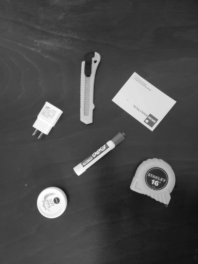
The grayscale image is shown in the figure below.
The next step is to threshold the image and convert it to binary form. We use the OpenCV function “cv2.threshold()” to threshold the image. We first perform the basic thresholding. The following code lines are used to threshold the image and convert it to a binary form.
# THRESHOLD
# https://docs.opencv.org/4.x/d7/d4d/tutorial_py_thresholding.html
#estimatedThreshold, thresholdImage=cv2.threshold(grayImage,50,255,cv2.THRESH_BINARY|cv2.THRESH_OTSU)
estimatedThreshold, thresholdImage=cv2.threshold(grayImage,90,255,cv2.THRESH_BINARY)
# display converted image
cv2.imshow('Image', thresholdImage)
cv2.waitKey(0)
cv2.destroyAllWindows()
cv2.imwrite("resizedPartsThreshold.png", thresholdImage, [cv2.IMWRITE_PNG_COMPRESSION, 0])
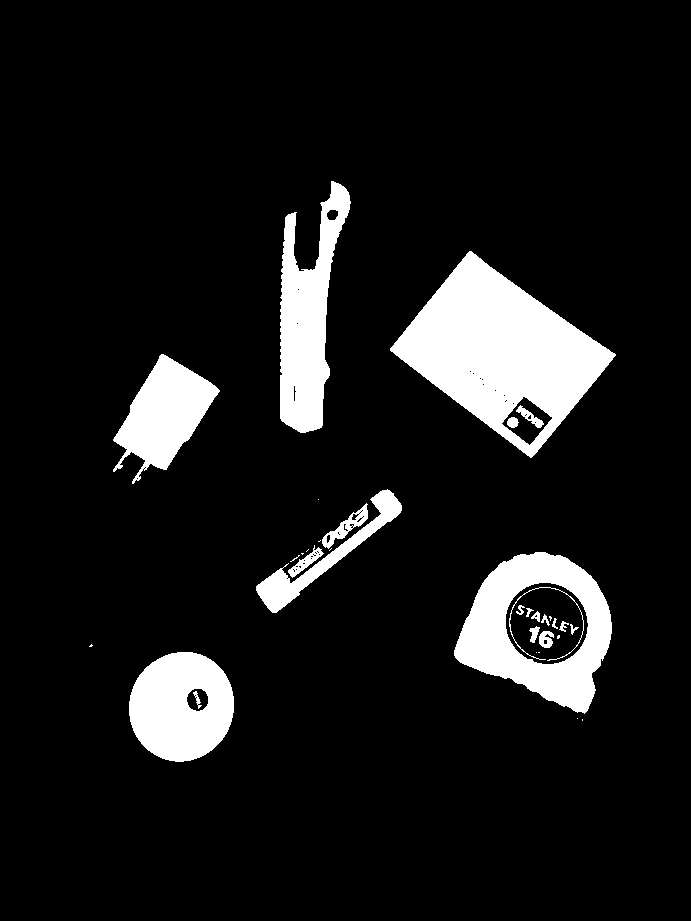
The function “cv2.threshold()” takes four arguments. The first argument is the image. The second value is the threshold value (in our case 90). The third argument is the value that is assigned to an image pixel that exceeds the threshold (in our case 255). The fourth argument is the threshold flag. In our case, this flag is “cv2.THRESH_BINARY”, indicating that we want to use binary thresholding. Here it should be noted that image pixel values that are smaller than the threshold value become equal to 0 after the threshold operation. This function returns two arguments. The first argument is the used threshold value, and the second argument is the resulting image. For details about the function “cv2.threshold”, see the official OpenCV tutorial page that can be accessed here. The thresholded image is shown in the figure below.

The following code lines are used to plot the histogram of the grayscale and thresholded image.
# PLOT HISTOGRAM OF THRESHOLDED AND GRAYSCALE IMAGES
plt.figure(figsize=(14, 12))
plt.subplot(2,2,1), plt.imshow(grayImage,'gray'), plt.title('Grayscale Image')
plt.subplot(2,2,2), plt.hist(grayImage.ravel(), 256), plt.title('Color Histogram of Grayscale Image')
plt.subplot(2,2,3), plt.imshow(thresholdImage,'gray'), plt.title('Binary (Thresholded)  Image')
plt.subplot(2,2,4), plt.hist(thresholdImage.ravel(),256), plt.title('Color Histogram of Binary (Thresholded) Image')
plt.savefig('fig1.png')
plt.show()
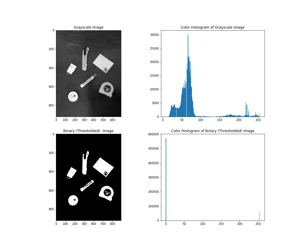
The results are shown in the figure below.

From Fig. 4, we can observe the histograms of the grayscale and thresholded image.
The second argument (threshold value) of the function “cv2.threshold()” has to be properly tuned since its value has a significant influence on the performance of the contour detection algorithm. Instead of guessing this parameter, we can also try another threshold method. That is, instead of allowing the user to select the threshold parameter, an algorithm can determine the threshold value. We can use Otsu’s method that automatically selects the threshold parameter. The following code lines are used to perform Otsu’s automatic thresholding.
# THRESHOLD
# https://docs.opencv.org/4.x/d7/d4d/tutorial_py_thresholding.html
estimatedThreshold, thresholdImage=cv2.threshold(grayImage,50,255,cv2.THRESH_BINARY|cv2.THRESH_OTSU)
#estimatedThreshold, thresholdImage=cv2.threshold(grayImage,90,255,cv2.THRESH_BINARY)
# display converted image
cv2.imshow('Image', thresholdImage)
cv2.waitKey(0)
cv2.destroyAllWindows()
cv2.imwrite("resizedPartsThreshold.png", thresholdImage, [cv2.IMWRITE_PNG_COMPRESSION, 0])
The result is shown in the figure below.
By comparing Figures 3 and 5, we can observe that in Fig. 5 small white areas are almost completely filtered. The following code line
estimatedThreshold, thresholdImage=cv2.threshold(grayImage,50,255,cv2.THRESH_BINARY|cv2.THRESH_OTSU)
performs Otsu’s thresholding. We last argument “cv2.THRESH_BINARY|cv2.THRESH_OTSU” tells to the function cv2.threshold() to use the Otsu’s method. This function now returns (as the first output) an estimate of the threshold value that is computed by Otsu’s algorithm. In our case, this value is: 133.
The histograms produced by Otsu’s method are shown below (compare these results with Fig. 4).
The following code lines are used to detect contours and display them.
## DETERMINE CONTOURS AND FILTER THEM
contours, hierarchy = cv2.findContours(thresholdImage,cv2.RETR_CCOMP,cv2.CHAIN_APPROX_SIMPLE)

#make a copy of the resized image since we are going to draw contours on the resized image
resizedImageCopy=np.copy(resizedImage)

# draw all contours with setting the parameter to -1
# but if you use this function, you should comment the for loop below
#cv2.drawContours(resizedImageCopy,contours,-1,(0,0,255),2)
#filter contours
for i, c in enumerate(contours):
    areaContour=cv2.contourArea(c)
    if areaContour<2000 or 100000<areaContour:
        continue
    cv2.drawContours(resizedImageCopy,contours,i,(255,10,255),4)

# display the original image with contours
cv2.imshow('Image', resizedImageCopy)
cv2.waitKey(0)
cv2.destroyAllWindows()
cv2.imwrite("resizedPartsContours.png", resizedImageCopy, [cv2.IMWRITE_PNG_COMPRESSION, 0])
The following code line is used to determine the contours
cv2.findContours(thresholdImage,cv2.RETR_CCOMP,cv2.CHAIN_APPROX_SIMPLE)
Detailed explanations of this function can be found here, here, and here.
The first argument is the thresholded image. The second argument “cv2.RETR_CCOMP” indicates contour retrieval mode. According to the OpenCV documentation that can be found here, this flag finds all the contours and organizes them in a 2-level hierarchy.
According to the OpenCV documentation that can be found here, the third argument “cv2.CHAIN_APPROX_SIMPLE” removes the unnecessary points and thus it saves the memory. Since this is a beginner-level tutorial, we will not explain other options. The function “cv2.findContours” returns two objects. The first object contains the computed contours, and the second object contains information about contour hierarchy. We only need the first output “contours”.
In code line 5 we make a copy of the resized color image since we want to display the contours on the color image, and we do not want to ruin our original resized image. The commented code line 9 is used to add all the contours to the image. We commented this line since we want to filter (remove) small contours and contours that are too large. The for loop in the code lines 11-15 is used to add the contours to the image. We do not add contours that are too small or too large (if statement that filters contours according to the inner area that they describe). The following code line
cv2.drawContours(resizedImageCopy,contours,i,(255,10,255),4)
is used to add contours to the image. The third argument denotes the contour index, the fourth argument (255,10,255) is the color of the contour, and the last argument is the contour thickness. It should be noted that this function does not display the contours. Instead, it only adds a contour to the image. The remaining code lines are used to display the image with contours.
Figure 7 below shows the contours obtained for the manually selected threshold parameter. Figure 8 shows the contours when the threshold parameter is selected by using Otsu’s method.
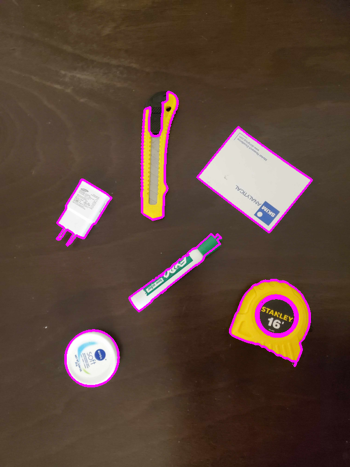
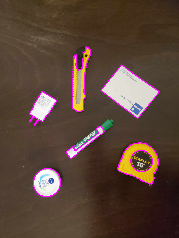
We can observe that manual thresholding produces better results than Otsu’s method since in Fig. 8, the marker contours are not properly detected (green parts of the marker are not properly included in the contour). However, the manually selected value of 90 is selected by trial and error.