Solve Ordinary Differential Equations in Python by Using odeint() Function – Fusion of Engineering, Control, Coding, Machine Learning, and Science

In this tutorial, we will learn how to solve Ordinary Differential Equations (ODEs) in Python by using the odeint() function. The YouTube page accompanying this tutorial is given below.

Test Problem – Pendulum Ordinary Differential Equation

In this tutorial, we consider the following ODE, describing the dynamics of the pendulum system. In our previous post, whose link can be found here, we explained how to derive this equation. The equation takes the following form

(1) $\begin{align*}\ddot{\alpha}+k_{1}\dot{\alpha}+k_{2}\sin(\alpha)=0\end{align*}$

where $\alpha$ is an angle or rotation measured from the vertical axis and $k_{1}$ and $k_{2}$ are constants, and the dots above variables denote first or second derivatives with respect to time.

State-space Form of Ordinary Differential Equation

The first step that needs to be performed when solving ODEs is to transform an ODE into a system of first-order differential equations. That is, the first step is to transform the ODE into a state-space form. We introduce state-space variables as follows

(2) $\begin{align*}& x_{1}=\alpha \\& x_{2}=\dot{\alpha}\end{align*}$

where $x_{1}$ and $x_{2}$ are new variables called the state-space variables. By using these newly introduced variables, and by using the ODE (1), we can write

(3) $\begin{align*}& \dot{x}_{1}=x_{2} \\& \dot{x}_{2}= - k_{1}x_{2}-k_{2}\sin(x_{1})\end{align*}$

The last equation can be written compactly

(4) $\begin{align*}\dot{\mathbf{x}}=\mathbf{f}(\mathbf{x})\end{align*}$

where $\mathbf{x}\in \mathbb{R}^{2}$ is the state vector and $\mathbf{f}(\mathbf{x})$ is a nonlinear vector function defined by

(5) $\begin{align*}& \mathbf{x}=\begin{bmatrix}x_{1} \\ x_{2} \end{bmatrix} \\& \mathbf{f}(\mathbf{x})=\begin{bmatrix} x_{2} \\ - k_{1}x_{2}-k_{2}\sin(x_{1}) \end{bmatrix}\end{align*}$

Solution of the Problem by Using the odeint() Python Function

The first step is to import the necessary libraries

import numpy as np
from scipy.integrate import odeint
import matplotlib.pyplot as plt

First, we import the NumPy library. Then we import the odeint() function from scipy.integrate. The SciPy library provides algorithms for numerical analysis, optimization, and integration of differential equations. Finally, we import the plotting tools.

Next, we need to define a Python function that will represent our ODE. This function is defined by the following code lines

def rightSideODE(x,t,k1,k2):
    dxdt=[x[1],-k1*x[1]-k2*np.sin(x[0])]
    return dxdt

Basically, the first argument is “x”. It is a row vector representing the state-space variables $x_{1}$ and $x_{2}$ . These are the dependent variables. The second argument is time $t$ . This is an independent variable. The last two arguments $k_{1}$ and $k_{2}$ are the constants defining our ODE. This function should compute and return the right-hand side of the equation (4). That is, the right-hand side of our state-space model. The right hand-side is defined by

[x[1],-k1*x[1]-k2*np.sin(x[0])]

Once we have defined our ODE, we need to define the initial condition, integration time points, and the constants $k_{1}$ and k_{2}. This can be done by using the following code lines:

# set the initial conditions
x0=[0,1]

# define the discretization points
timePoints=np.linspace(0,100,300)

#define the constants 
k1=0.1
k2=0.5

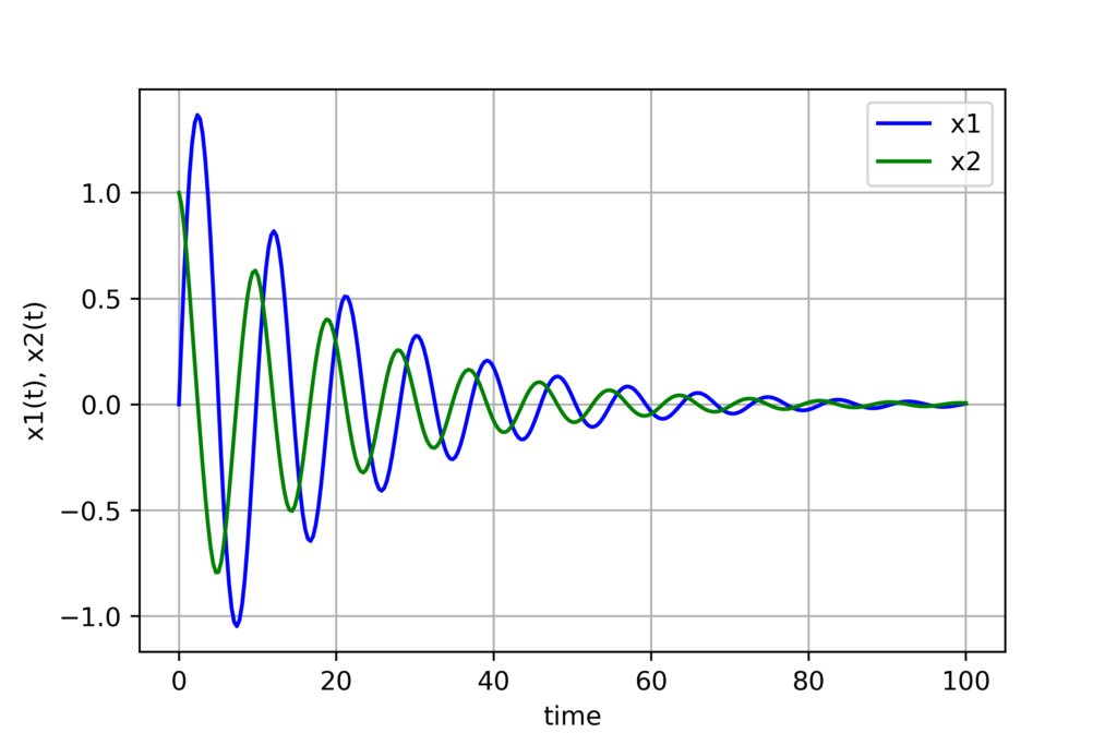
Finally, we call the odeint() function and plot the results:

solutionOde=odeint(rightSideODE,x0,timePoints, args=(k1,k2))

plt.plot(timePoints, solutionOde[:, 0], 'b', label='x1')
plt.plot(timePoints, solutionOde[:, 1], 'g', label='x2')
plt.legend(loc='best')
plt.xlabel('time')
plt.ylabel('x1(t), x2(t)')
plt.grid()
plt.savefig('simulation.png')
plt.show()

The main part of this code is the function call:

solutionOde=odeint(rightSideODE,x0,timePoints, args=(k1,k2))

The first argument is the name of the function that defines the ODE. In our case, the name of the function is “rightSideODE”. The second argument is the row vector x0 defining the initial conditions. The third argument is the row vector containing time points at which the solution is computed. The final argument contains the constants $k_{1}$ and k_{2}. This code produced the following graph.

Figure 1: Simulated state trajectories of the pendulum ODE.

The complete code used in this post is given below.

# -*- coding: utf-8 -*-
"""
Created on Mon Oct 10 18:27:57 2022

@author: aleks
"""

import numpy as np
from scipy.integrate import odeint
import matplotlib.pyplot as plt


def rightSideODE(x,t,k1,k2):
    dxdt=[x[1],-k1*x[1]-k2*np.sin(x[0])]
    return dxdt

# set the initial conditions
x0=[0,1]

# define the discretization points
timePoints=np.linspace(0,100,300)

#define the constants 
k1=0.1
k2=0.5

solutionOde=odeint(rightSideODE,x0,timePoints, args=(k1,k2))

plt.plot(timePoints, solutionOde[:, 0], 'b', label='x1')
plt.plot(timePoints, solutionOde[:, 1], 'g', label='x2')
plt.legend(loc='best')
plt.xlabel('time')
plt.ylabel('x1(t), x2(t)')
plt.grid()
plt.savefig('simulation.png')
plt.show()

Test Problem – Pendulum Ordinary Differential Equation

State-space Form of Ordinary Differential Equation

Solution of the Problem by Using the odeint() Python Function

admin

You might also like

Solve a System of Nonlinear Equations in MATLAB

Solve Systems of Nonlinear Equations in Python by Using FSOLVE

Rotation Matrix Tutorial for Robotics and Aerospace Engineering – Rotation Matrix Around X Axis