Derivation and Explanation of the Formula for Settling Time of Transient Response – Fusion of Engineering, Control, Coding, Machine Learning, and Science

In this tutorial and in the accompanying YouTube video, we derive and explain the formula for the settling time of the transient response of a dynamical system. This formula is important since it relates the settling time with the natural undamped frequency and damping ratio. Also, it can be used to design controllers that meet certain transient response specifications. The YouTube video accompanying this post is given below.

Final expression

In this post, we show that the settling time of the transient response can be approximated by the following equation

(1) $\begin{align*}t_{s} \approx \frac{4}{\zeta \omega_{n}}\end{align*}$

where $t_{s}$ is the settling time, $\zeta$ is the damping ratio, and $\omega_{n}$ is the natural undamped frequency.

Derivation of the formula for the settling time

The prototype second-order system has the following form:

(2) $\begin{align*}W(s)=\frac{\omega_{n}^{2}}{s^2+2\zeta \omega_{n} s +\omega_{n}^{2}}\end{align*}$

where

$s$ is the complex variable
$\omega_{n}$ is the natural undamped frequency
$\zeta$ is the damping ratio

When deriving the formulas, we assume that the input of the system is a step signal. The output is then

(3) $\begin{align*}Y(s)=W(s)U(s), \;\;\; U(s)=\frac{1}{s}\end{align*}$

In our previous post, which can be found here, we derived an analytical form of the step response in the time domain. The response has the following form

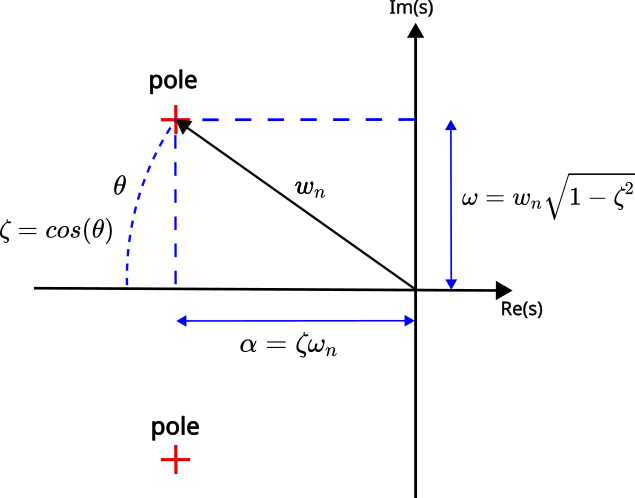
(4) $\begin{align*}y(t)& =1- \frac{e^{-\zeta \omega_{n} t}}{\sqrt{1-\zeta^2}} \sin((\omega_{n} \sqrt{1-\zeta^2}) t +\cos^{-1}(\zeta))\end{align*}$

With this formula, it is always a good idea to give the following figure (see below) that illustrates the poles of the prototype system (2). A detailed explanation of this figure can be found in our previous post that can be found here.

Figure 1: Poles of a second-order prototype system.

Let us now analyze the equation (4). The envelopes of the transient response are given by the following exponential functions

(5) $\begin{align*}a_{1}(t)&=1+\frac{e^{-\zeta \omega_{n} t}}{\sqrt{1-\zeta^2}} \\a_{2}(t)&=1-\frac{e^{-\zeta \omega_{n} t}}{\sqrt{1-\zeta^2}}\end{align*}$

The step response of the system with the two envelopes are shown in the figure below.

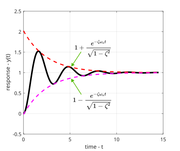
Figure 2: Step response of the system with two envelopes that bound the damped oscillations.

This graph is generated by using the following MATLAB code.

zeta=0.2
wn=2
transferFunction= tf([wn^2],[1 2*zeta*wn wn^2])

[y,time1]=step(transferFunction);
  
% create the envelopes

upperEnvelope=1+exp(-zeta*wn*time1)/(sqrt(1-zeta^2));
lowerEnvelope=1-exp(-zeta*wn*time1)/(sqrt(1-zeta^2));

figure(1)
hold on
plot(time1,y,'k')
plot(time1,upperEnvelope,'r')
plot(time1,lowerEnvelope,'m')

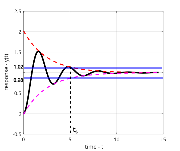
The settling time is defined in our previous post which can be found here. Formally speaking, the settling time is defined as follows.

Definition of $\pm 2 \%$ settling time: The settling time $t_{s}$ is defined as the time required for the transient response to enter and stay within $\pm 2\%$ of the steady-state or final value.

We can approximately determine the settling time by solving the following equation that is based on the envelope function of the transient response:

(6) $\begin{align*}1+\frac{e^{-\zeta \omega_{n} t_{s}}}{\sqrt{1-\zeta^2}}=1.02\end{align*}$

This approximation is illustrated in the figure below.

Figure 3: Approximation of the settling time by using the envelopes of the transient response.

From (6), we obtain

(7) $\begin{align*}\frac{e^{-\zeta \omega_{n} t_{s}}}{\sqrt{1-\zeta^2}} & =0.02 \\-\zeta \omega_{n} t_{s} & = \ln (0.02 \sqrt{1-\zeta^2}) \\t_{s} & = - \frac{\ln (0.02 \sqrt{1-\zeta^2})}{\zeta \omega_{n}}\end{align*}$

That is, we obtained the following approximation

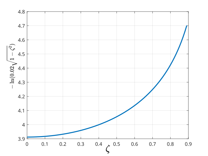
(8) $\begin{align*}t_{s} & = - \frac{\ln (0.02 \sqrt{1-\zeta^2})}{\zeta \omega_{n}}\end{align*}$

This equation is quite complex, and let us try to simplify this equation. Figure below shows the term $-\ln (0.02 \sqrt{1-\zeta^2})$ with respect to the parameter $\zeta$ . As the parameter $\zeta$ is varied from $0.001$ to $0.9$ , the term $-\ln (0.02 \sqrt{1-\zeta^2})$ varies from $3.91$ to $4.7$ . This variation is illustrated in the figure below.

Figure 4: Variation of the term $-\ln (0.02 \sqrt{1-\zeta^2})$ with respect to the parameter $\zeta$ .

This graph is generated by using the following MATLAB code

zeta=0.001:0.01:0.9

y=-log(0.02*sqrt(1-zeta.^2))

plot(zeta,y)

From this graph, we can observe that we can approximate the term $-\ln (0.02 \sqrt{1-\zeta^2})$ as follows

(9) $\begin{align*}-\ln (0.02 \sqrt{1-\zeta^2}) \approx 4\end{align*}$

By substituting this approximation in (8), we can obtain our final expression for the approximation of the settling time:

(10) $\begin{align*}t_{s} \approx \frac{4}{\zeta \omega_{n}}\end{align*}$

Final expression

Derivation of the formula for the settling time

admin

You might also like

Matrix Exponential Tutorial: Definition, Calculation, and its Application in Control Engineering and Control Theory – PART 1

Convert State-Space Models into Transfer Functions with MATLAB Codes

Matrix Minor, Matrix Cofactor, Adjugate Matrix, and Formula for Matrix Inversion – Linear Algebra Tutorial