Transient Response Specifications: Peak time, Settling time, Rise Time, Overshoot, and Percent Overshoot – Fusion of Engineering, Control, Coding, Machine Learning, and Science

1. Introduction

In this post and in the accompanying YouTube tutorial, we provide explanations of transient response specifications: peak time, settling time, rise time, overshoot, and percent overshoot. The YouTube video accompanying this post is given below.

The values of peak time, settling time, rise time, and percent overshoot are very important for control design. We often specify the desired system behavior in terms of the values of these parameters of the transient response. Then, on the basis of the desired values of these parameters, we design the control system. Also, for second-order systems, we can relate damping ratio, natural frequency, bandwidth, and some other properties of the dynamical systems with the values of peak time, settling time, rise time, and percent overshoot.

In this post, we formally define the peak time, settling time, rise time, and percent overshoot and we provide graphical explanations of these important parameters.

The step response that is shown in the figures below is computed for the following system

(1) $\begin{align*}W(s)=\frac{4}{s^2+1.6s+4}\end{align*}$

The step response is computed by using the following MATLAB code

zeta=0.4
wn=2
transferFunction= tf([wn^2],[1 2*zeta*wn wn^2])

[y,time1]=step(transferFunction)

plot(time1,y)

2. Settling time

Settling time, denoted by $t_{s}$ is graphically explained in Fig. 1. below. The final or steady-state value of the system response is denoted by $y_{ss}$ .

Figure 1: Explanation of the settling time of a dynamical system.

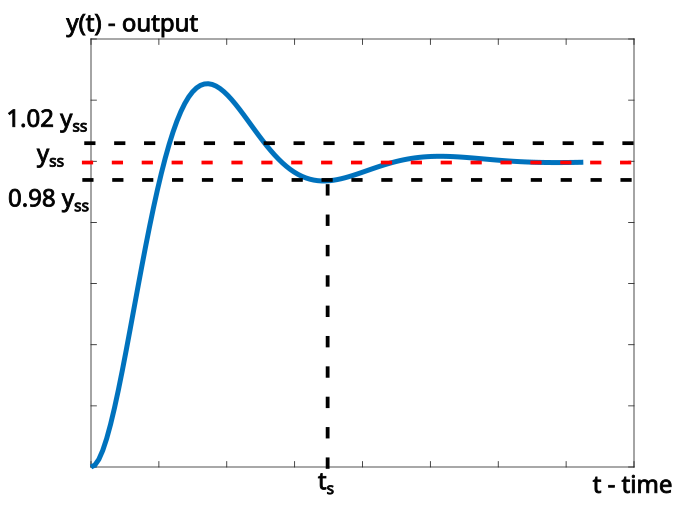
Definition of $\pm 2 \%$ settling time: The settling time $t_{s}$ is defined as the time required for the transient response to enter and stay within $\pm 2\%$ of the steady-state or final value.

Here are a few important comments about the settling time. First of all, in a similar manner and spirit to the above definition, we can also define $\pm 5\%$ settling time. Then, obviously, the definition of the settling time implicitly assumes that the system reaches a finite steady state. This implicitly implies that the underlying system is asymptotically stable. As is demonstrated in Fig. 1, we can construct the settling time by first drawing a horizontal line starting from the steady-state value of the response. Then, we offset this line $\pm 2\%$ to obtain an interval or a tunnel. Then we search for an intersection of the system response with the $\pm 2\%$ horizontal line such that the response enters and never leaves the tunnel after the intersection point. The time corresponding to the intersection point is our settling time.

Finally, the settling time, as well as other transient response parameters defined in this post can also be defined for not only second-order systems but for systems of arbitrary orders.

3. Peak Time

The peak time is another important characteristic of the transient system response. It is usually defined as follows:

Definition of the peak time: The peak time, denoted by $t_{p}$ is defined as the time required for the system to reach the maximum overshoot.

The peak time is illustrated in Fig. 2. below.

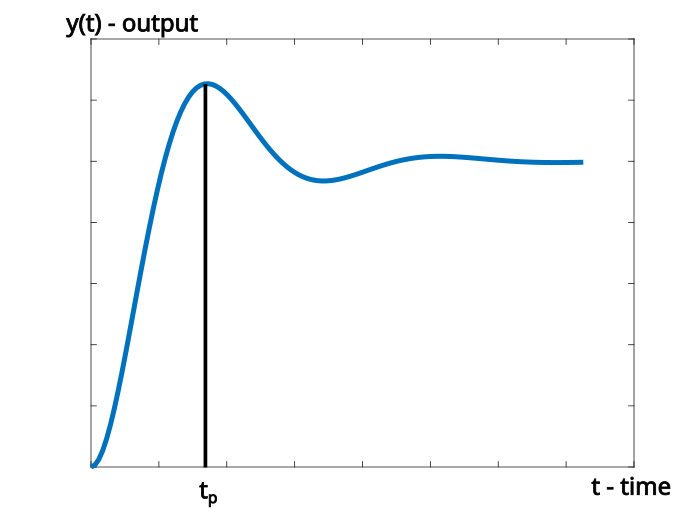
Figure 2: Graphical explanation of the peak time of the transient response.

4. Rise Time

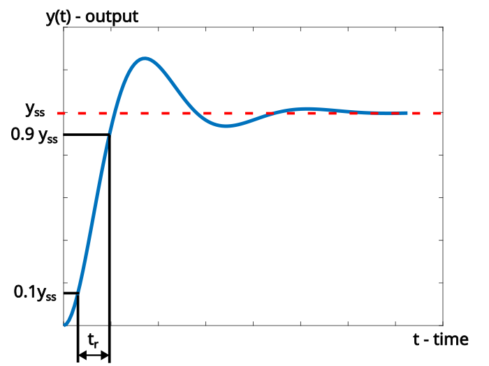
Definition of the rise time: The rise time is the time required for the system response to go from $10 \%$ to $90 \%$ of its final or steady-state value.

The rise time is explained in Fig. 3 below. The final or steady-state value of the system response is denoted by $y_{ss}$ . $10\%$ and $90\%$ of the final values are denoted by $0.1y_{ss}$ and $0.9 y_{ss}$ , respectively.

Figure 3: Graphical explanation of the rise time of the system transient response.

5. Overshoot and percentage overshoot

The maximum overshoot can be defined as follows:

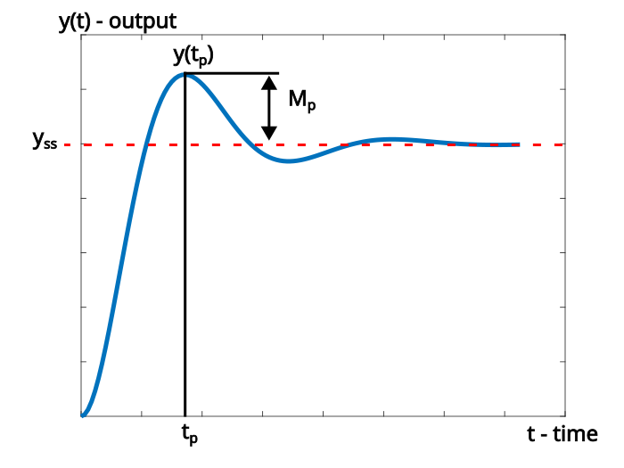
Definition of the (maximum) overshoot: The (maximum) overshoot, denoted by $M_{p}$ is defined by

(2) $\begin{align*}M_{p}=y(t_{p})-y_{ss}\end{align*}$

where $t_{p}$ is the peak time for which the step response achieves a maximum value, and $y_{ss}$ is the final or the steady value of the step response. The (maximum) overshoot is illustrated in Fig. 4 below.