Equations of Motion of a Pendulum on a Cart by Using Lagrange’s Equations – Fusion of Engineering, Control, Coding, Machine Learning, and Science

In this dynamics tutorial, we explain how to derive the equations of motion (model) of a pendulum on a cart. We use Lagrange’s equations to derive the model. For brevity, in this tutorial, we call our system the cart-pendulum system. The YouTube tutorial accompanying this webpage tutorial is given below.

Before we start with derivations, let us first explain the main motivation for deriving the model of the cart-pendulum system. First of all, the cart-pendulum system is a classical nonlinear dynamical system that is often used to benchmark different linear and nonlinear estimation and control methods. Also, it is often used in the machine learning community to benchmark different machine learning and reinforcement learning algorithms. Finally, the cart-pendulum system is a starting point for modeling a number of real systems, such as self-balancing scooters (segway vehicles), rockets, bipedal robots, human biomechanics, sloshing of fuel in spacecraft, etc.

In this tutorial, we derive an equation of motion of the cart-pendulum system. In the second part of this tutorial, given here, we explain how to automatically derive a state-space model of this system in Python and how to simulate the state-space model in Python. In the third part of this tutorial, given here, we explain how to use the simulated state-space trajectories to animate the motion of the system by using Python’s Pygame library.

The YouTube video of the second tutorial part:

The YouTube video of the third tutorial part:

Derivation of Equation of Motion of Cart-Pendulum Mechanical System

Consider the figure shown below.

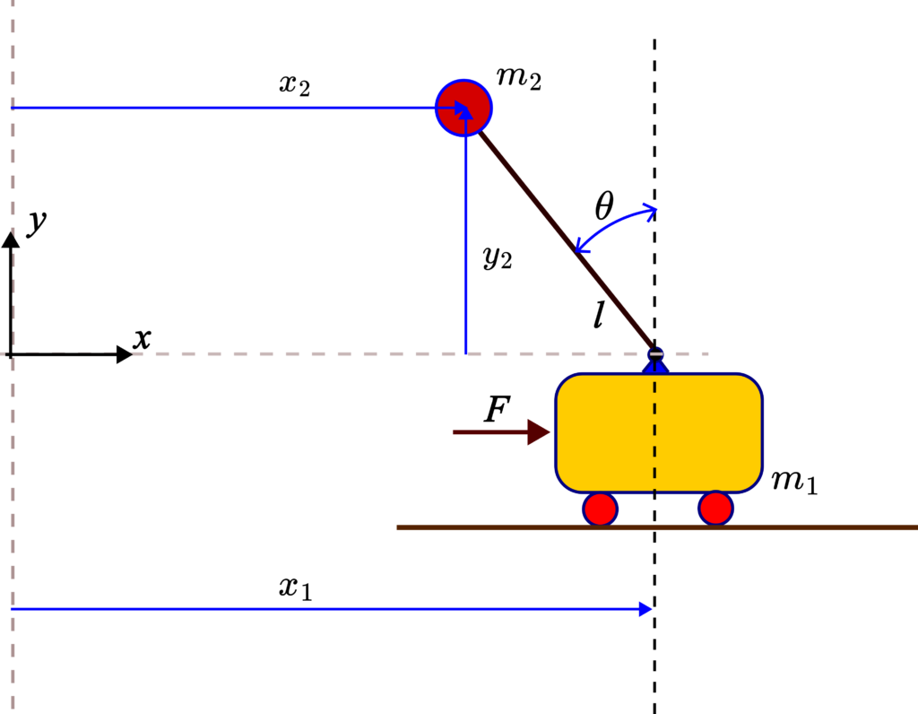
The system consists of a cart with a mass of $m_{1}$ that is driven by the force $F$ . Point mass $m_{2}$ is rigidly attached to the rod of length $l$ . The system consisting of the rod and the point mass is called the pendulum. The pendulum can freely rotate since it is supported by a rotating support that is attached to the cart. We neglect the mass of the rod (there are also models that model the rod’s rigid body dynamics, however, in this tutorial, we do not consider such models). The horizontal distances of the cart and the point mass from the $y$ axis are denoted by $x_{1}$ and $x_{2}$ , respectively. The vertical distance of the point mass to the $x$ axis is denoted by $y_{2}$ . The angle $\theta$ is the angle that the pendulum makes with respect to the vertical axis, and the positive angle is in the counter-clock direction.

To model the system, we first need to select the so-called generalized coordinates. The generalized coordinates are usually selected as a set of independent coordinates or variables that uniquely define the configuration of the system. In our case, these generalized coordinates are $x_{1}$ and $\theta$ . Obviously, if we fix $x_{1}$ and $\theta$ , the configuration of the system is uniquely determined. Here, since we do not have additional constraints, $x_{1}$ and $\theta$ can be seen as the degrees of freedom of the system.

To derive Langrange’s equations, we first need to derive the expressions for the kinetic and potential energies of the system. Consequently, the next step is to derive the expressions for the kinetic and potential energy of the system in terms $x_{1}$ and $\theta$ . The kinetic energy can be represented as follows

(1) $\begin{align*}E_{k}=E_{k1}+E_{k2}\end{align*}$

where $E_{k1}$ is the kinetic energy of the cart and $E_{k2}$ is the kinetic energy of the point mass. The kinetic energy of the cart is easy to compute due to the fact that the cart is only translating along the x-axis:

(2) $\begin{align*}E_{k1}=\frac{1}{2}m_{1}v_{1}^{2}=\frac{1}{2}m_{1}\dot{x}^{2}_{1}\end{align*}$

where the magnitude of the velocity of the cart is denoted by $v_{1}$ and we have

(3) $\begin{align*}v_{1}=\dot{x}_{1}\end{align*}$

where $\dot{x}_{1}$ is the time derivative of the cart position $x_{1}$ . That is $\dot{x}_{1}=\frac{dx_{1}}{dt}$ . The expression for the kinetic energy of the point mass is more complex. The kinetic energy is defined by

(4) $\begin{align*}E_{k2}=\frac{1}{2}m_{2}v_{2}^{2}\end{align*}$

where $v_{2}$ is the magnitude of the velocity of the cart. The magnitude of this velocity is given by

(5) $\begin{align*}v_{2}^{2}=v_{2x}^{2}+v_{2y}^{2}\end{align*}$

where $v_{2x}$ and $v_{2y}$ are the $x$ and $y$ components of the velocity vector, defined by

(6) $\begin{align*}v_{2x}=\dot{x}_{2} \\v_{2y}=\dot{y}_{2} \end{align*}$

To compute these velocity components, we need to find the expressions for $x_{2}$ and $y_{2}$ . From Fig.1., we have

(7) $\begin{align*}x_{2}=x_{1}-l\sin(\theta) \\y_{2}=l\cos(\theta)\end{align*}$

By differentiating the previous expressions with respect to time, we obtain

(8) $\begin{align*}\dot{x}_{2}&=\dot{x}_{1}-l\dot{\theta}\cos(\theta) \\\dot{y}_{2}&=-l\dot{\theta}\sin(\theta)\end{align*}$

By substituting (6) and (8) in (5) and later on in (4), we obtain

(9) $\begin{align*}E_{k2} & = \frac{1}{2}m_{2}\Big( \big(\dot{x}_{1}-l\dot{\theta}\cos(\theta) \big)^{2}+\big( -l\dot{\theta}\sin(\theta) \big)^{2} \Big) \\&=\frac{1}{2}m_{2}\Big( \dot{x}_{1}^{2}-2l\dot{x}_{1}\dot{\theta}\cos(\theta)+l^{2}\dot{\theta}^{2}\Big) \end{align*}$

By combining (9) and (2), we obtain the final expression for the kinetic energy

(10) $\begin{align*}E_{k}=\frac{1}{2}\big(m_{1}+m_{2}\big)\dot{x}_{1}^{2}-m_{2}l\dot{x}_{1}\dot{\theta}\cos(\theta)+\frac{1}{2}m_{2}l^{2}\dot{\theta}^{2}\end{align*}$

The potential energy of the system is the potential energy of the point mass that is defined by

(11) $\begin{align*}E_{p}=m_{2}gl\cos(\theta)\end{align*}$

where $g$ is the gravitational acceleration constant, and $l\cos(\theta)$ is the distance of the point mass to the zero-level of the potential energy. In our case, the zero level is defined by $y=0$ .

Next, we define Lagrange’s equations. In our case, Lagrange’s equations are defined by

(12) $\begin{align*}\frac{d}{dt}\Big(\frac{\partial L}{\partial \dot{x}_{1}} \Big)-\frac{\partial L}{\partial x_{1}} & =F \\\frac{d}{dt}\Big(\frac{\partial L}{\partial \dot{\theta}} \Big)-\frac{\partial L}{\partial \theta} & =0 \end{align*}$

where $L$ is the Lagrangian defined by

(13) $\begin{align*}L=E_{k}-E_{p}\end{align*}$

By substituting (10) and (11) in (13), we obtain the final expression for the Lagrangian

(14) $\begin{align*}L= \frac{1}{2}\big(m_{1}+m_{2}\big)\dot{x}_{1}^{2}-m_{2}l\dot{x}_{1}\dot{\theta}\cos(\theta)+\frac{1}{2}m_{2}l^{2}\dot{\theta}^{2}-m_{2}gl\cos(\theta)\end{align*}$

The last equation defines the Lagrangian of the system. Next, in order to derive the equations of motion, we need to compute the derivatives in (12). We have

(15) $\begin{align*}\frac{\partial L}{\partial \dot{x}_{1}}=\big(m_{1}+m_{2}\big)\dot{x}_{1}-m_{2}l\dot{\theta}\cos(\theta) \end{align*}$

(16) $\begin{align*}\frac{d}{dt}\Big( \frac{\partial L}{\partial \dot{x}_{1}} \Big)=\big(m_{1}+m_{2} \big)\ddot{x}_{1}-m_{2}l\ddot{\theta}\cos(\theta)+m_{2}l\dot{\theta}^{2}\sin(\theta)\end{align*}$

(17) $\begin{align*}\frac{\partial L}{\partial x_{1}}=0\end{align*}$

By substituting (16) and (17) in the first equation of (12), we obtain the first equation of motion

(18) $\begin{align*}\big(m_{1}+m_{2} \big) \ddot{x}_{1}-m_{2}l\ddot{\theta}\cos(\theta)+m_{2}l\dot{\theta}^{2}\sin(\theta)=F\end{align*}$

To obtain the second equation of motion, we compute the following partial derivatives

(19) $\begin{align*}\frac{\partial L}{\partial \dot{\theta}}=-m_{2}l\dot{x}_{1}\cos(\theta)+m_{2}l^{2}\dot{\theta}\end{align*}$

(20) $\begin{align*}\frac{d}{dt}\Big( \frac{\partial L}{\partial \dot{\theta}}\Big)=-m_{2}l\ddot{x}_{1}\cos(\theta)+m_{2}l\dot{x}_{1}\dot{\theta}\sin(\theta)+m_{2}l^{2}\ddot{\theta}\end{align*}$

(21) $\begin{align*}\frac{\partial L}{\partial \theta} = m_{2}l\dot{x}_{1}\dot{\theta}\sin(\theta)+m_{2}gl\sin(\theta)\end{align*}$

By substituting (20) and (21) in the second equation of (12), we obtain

(22) $\begin{align*} -m_{2}l\ddot{x}_{1}\cos(\theta)+m_{2}l\dot{x}_{1}\dot{\theta}\sin(\theta)+m_{2}l^{2}\ddot{\theta}-m_{2}l\dot{x}_{1}\dot{\theta}\sin(\theta)-m_{2}gl\sin(\theta)=0\end{align*}$

From the last equation, we obtain

(23) $\begin{align*}-m_{2}l\ddot{x}_{1}\cos(\theta)+m_{2}l^{2}\ddot{\theta}-m_{2}gl\sin(\theta)=0\end{align*}$

By dividing the last equation with $m_{2}l$ , we obtain the second equation of motion

(24) $\begin{align*}l\ddot{\theta}-\ddot{x}_{1}\cos(\theta)-g\sin(\theta)=0\end{align*}$

The two equations of motion are summarized below for completeness

(25) $\begin{align*}& \big(m_{1}+m_{2} \big) \ddot{x}_{1}-m_{2}l\ddot{\theta}\cos(\theta)+m_{2}l\dot{\theta}^{2}\sin(\theta)=F \\& l\ddot{\theta}-\ddot{x}_{1}\cos(\theta)-g\sin(\theta)=0\end{align*}$

Derivation of Equation of Motion of Cart-Pendulum Mechanical System

admin

You might also like

Test 4

Calculate Magnitude and Phase of Transfer Functions and Practice Complex Number Transformations – Control Engineering Tutorials

Iterative Policy Evaluation Algorithm in Python (OpenAI Gym) – Reinforcement Learning Tutorial