Iterative Policy Evaluation Algorithm in Python (OpenAI Gym) – Reinforcement Learning Tutorial – Fusion of Engineering, Control, Coding, Machine Learning, and Science

In this tutorial, we explain how to implement an iterative policy evaluation algorithm in Python. This tutorial is part of a series of tutorials on reinforcement learning. The YouTube tutorial accompanying this post is given below.

Required Previous Knowledge

Before reading this tutorial you should go over the following tutorials:

Motivation

The iterative policy evaluation algorithm is used in reinforcement learning algorithms to iteratively calculate the value function in certain states.

Test Example

To test the performance of the iterative policy evaluation algorithm, we consider the Frozen Lake environment in OpenAI Gym. A detailed tutorial dedicated to the OpenAI Gym and Frozen Lake environment can be found here. This environment is illustrated in Fig. 1. below

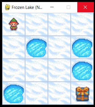
Figure 1: Illustration of the Frozen Lake environment.

This environment consists of 16 fields (4 by 4 grid). These fields are enumerated in the Figure 2 below.

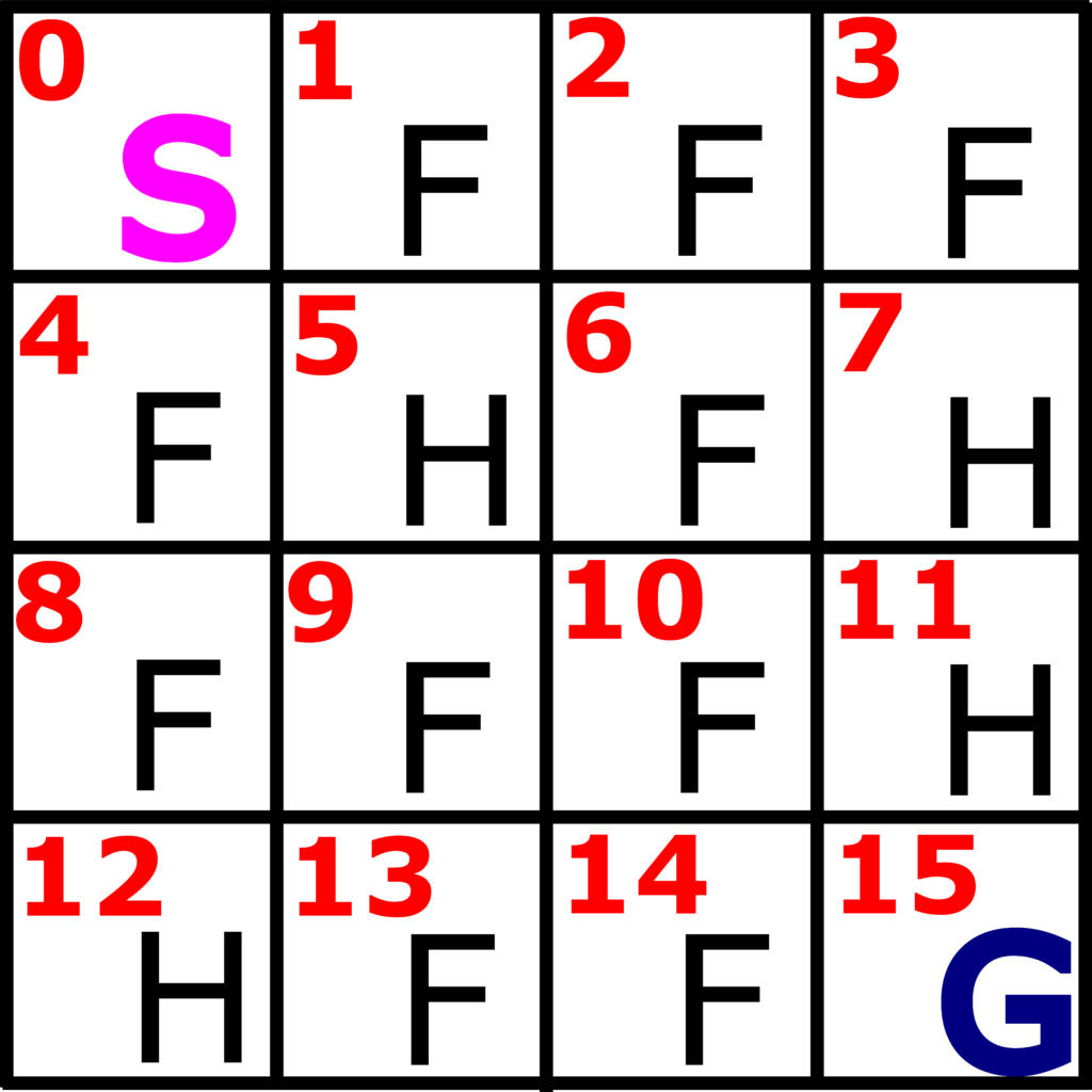
Figure 2: Enumeration of the fields of the Frozen Lake Environment.

There are four types of fields: start field (S), frozen fields (F), holes (H), and the goal field (G). The goal of the game is to reach the goal field G, starting from the start field S and by avoiding the hole fields. If the player steps on the frozen field, the player ends the game. That is, the game is completed if we step on a hole field or if we reach the goal field. A state or an observation is the current field. The states are denoted from 0 to 15.

We receive the reward of 0 if we step on the frozen or hole fields. On the other hand, we receive the reward of 1, if we step on the goal field. In any internal state (not close to the boundary) that is not a terminal state, we have 4 possible actions: UP, DOWN, LEFT, and RIGHT.

Brief Summary of the Value Function

Definition of the value function: The value function of a particular state $s$ under the policy $\pi$ , denoted by $v_{\pi}(s)$ , is the expectation of the return $G_{t}$ obtained by following the policy $\pi$ and starting from the state $s$ :

(1) $\begin{align*}v_{\pi}(s)=E_{\pi}[G_{t}|S_{t}=s]\end{align*}$

here $E_{\pi}[\cdot]$ denotes the expected value of the random variable $G_{t}$ obtained under the assumption that the agent follows the policy $\pi$ . The value function of the terminal state is defined to be zero. Also, the value function $v_{\pi}(s)$ is often called the state-value function for the policy $\pi$ .

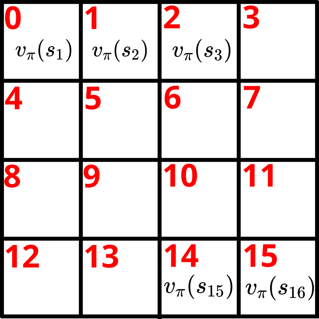
Let us consider again the Frozen lake example. To every field, that is, to every state $s_{1},s_{2},\ldots, s_{16}$ , we can associate the value function. This is shown in Fig. 3 below.

Figure 3: Value functions associated with states $s_{1}$ , $s_{2}$ , $s_{3}$ , $s_{15}$ , and $s_16$ .

A very important equation that enables us to iteratively compute the value function is the Bellman equation for the state value function $v_{\pi}(s)$ .

Bellman equation for the state value function $v_{\pi}(s)$ : Let $s'$ be the state at the time instant $t+1$ , and $s$ be the state at the time instant $s$ . Then, it can be shown that

(2) $\begin{align*}v_{\pi}(s) & =E_{\pi}[G_{t}|S_{t}=s] \\v_{\pi}(s) & = \sum_{a} \pi(a|s) \sum_{s'}\sum_{r}p(s',r|s,a)[r+\gamma v_{\pi}(s')]\end{align*}$

where

$r$ is the particular value of the reward obtained by reaching $s'$ and $v_{\pi}(s')$ is the state value function at $s'$ .
$a$ is the action performed in the state $s$
$\pi(a|s)$ is the (control) policy, that is, the probability of selecting action $a$ when in the state $s$
$p(s',r|s,a)$ is the dynamics of the Markov decision process:
(3) $\begin{align*}p(s',r|s,a)=\text{Probability}\{S_{t}=s',R_{t}=r| S_{t-1}=s, A_{t-1}=a \}\end{align*}$

Iterative Policy Evaluation Algorithm

The goal is to compute the value function $v_{\pi}(s)$ for every state expressed by using the Bellman equation

(4) $\begin{align*}v_{\pi}(s) & =E_{\pi}[G_{t}|S_{t}=s] \\v_{\pi}(s) & = \sum_{a} \pi(a|s) \sum_{s'}\sum_{r}p(s',r|s,a)[r+\gamma v_{\pi}(s')]\end{align*}$

Assuming that we have $N$ states $s$ , and by writing the Bellman equation for every state, we can obtain a system of linear equations where the unknowns are the states. By solving this system, we can compute the state value functions for every state. An alternative approach for computing the value functions is to use an iterative method. We can transform (4) into the following iteration:

(5) $\begin{align*}v_{\pi,k+1}(s) & = \sum_{a} \pi(a|s) \sum_{s'}\sum_{r}p(s',r|s,a)[r+\gamma v_{\pi,k}(s')]\end{align*}$

where $k$ is the iteration index, and $v_{\pi,k+1}(s)$ is the value function computed at the iteration $k+1$ and $v_{\pi,k}(s')$ is the value function computed at the iteration $k$ .

The iteration (5) is the core of the iterative policy evaluation algorithm. At the iteration $k=0$ , we simply initialize the iteration with a guess of the value functions $v_{\pi,0}(s)$ for every state, and we propagate the iteration until convergence. Here, it should be emphasized that the value functions for the terminal states (holes and the goal state in the Frozen Lake examples) should be initialized as zeros.

Let $\mathbf{v}_{k}$ , be the vector whose entries are value functions for the corresponding states. That is,

(6) $\begin{align*}\mathbf{v}_{k}=\begin{bmatrix} v_{\pi,k}(s_{1}) \\ v_{\pi,k}(s_{2}) \\ \vdots \\ v_{\pi,k}(s_{N}) \end{bmatrix}\end{align*}$

where $v_{\pi,k}(s_{i})$ is the value function at the state $s_{i}$ computed at the iteration $k$ . Then, we can stop the iteration when $\max(|\mathbf{v}_{k+1}- \mathbf{v}_{k} |) \le \delta$ , where $|\cdot|$ is an absolute value, and $\delta$ is the convergence tolerance (a relatively small number).

Python Implementation of the Iterative Policy Evaluation Algorithm

In our particular example, in (4) the sum over the rewards $r$ does not exist since the rewards are deterministic. That is, we always obtain the same rewards when reaching the final state $s'$ . That is, $p(s',r|s,a)=p(r|s,a)$ , where $p(r|s,a)$ is the transition probability. Consequently, iteration becomes

(7) $\begin{align*}v_{\pi,k+1}(s) & = \underbrace{\sum_{a} \pi(a|s) \underbrace{\sum_{s'}p(s'|s,a)[r+\gamma v_{\pi,k}(s')]}_{\text{inner sum}}}_{\text{outer sum}} \end{align*}$

Furthermore, in every state $s$ , we assume that all the actions are equally possible. That is $\pi(a_{i}|s)=0.25$ , $i=1,2,3,4$ (actions are UP, DOWN, LEFT, and RIGHT).

The first step is to import the necessary libraries and to import the Frozen Lake environment:

import gym
import matplotlib.pyplot as plt
import seaborn as sns
import numpy as no
 
env=gym.make("FrozenLake-v1", render_mode="human")
env.reset()
# render the environment
env.render()
env.close()

We can render the environment by calling env.render(). However, we do not need a graphical representation of the environment in this post. Consequently, we closed the graphical representation by typing: env.close().

We can inspect the observation space, action space, and transition probabilities by using these code lines

# observation space - states 
env.observation_space

# actions: left -0, down - 1, right - 2, up- 3
env.action_space


#transition probabilities
#p(s'|s,a) probability of going to state s' 
#          starting from the state s and by applying the action a

# env.P[state][action]
env.P[0][1] #state 0, action 1
# output is a list having the following entries
# (transition probability, next state, reward, Is terminal state?)

The iterative policy evaluation is implemented as follows

# select the discount factor
discountFactor=0.9
# initialize the value function vector
valueFunctionVector=np.zeros(env.observation_space.n)
# maximum number of iterations
maxNumberOfIterations=1000
# convergence tolerance delta
convergenceTolerance=10**(-6)

# convergence list 
convergenceTrack=[]

for iterations in range(maxNumberOfIterations):
    convergenceTrack.append(np.linalg.norm(valueFunctionVector,2))
    valueFunctionVectorNextIteration=np.zeros(env.observation_space.n)
    for state in env.P:
        outerSum=0
        for action in env.P[state]:
            innerSum=0
            for probability, nextState, reward, isTerminalState in env.P[state][action]:
                #print(probability, nextState, reward, isTerminalState)
                innerSum=innerSum+ probability*(reward+discountFactor*valueFunctionVector[nextState])
            outerSum=outerSum+0.25*innerSum
        valueFunctionVectorNextIteration[state]=outerSum
    if(np.max(np.abs(valueFunctionVectorNextIteration-valueFunctionVector))<convergenceTolerance):
        valueFunctionVector=valueFunctionVectorNextIteration
        print('Converged!')
        break
    valueFunctionVector=valueFunctionVectorNextIteration

This implementation closely follows (7). We have 3 for loops. The first loop iterates through all the states. The second for loop is the outer loop in (7) . The third loop is the inner loop in the same equations. The vector (6) is implemented as valueFunctionVector.

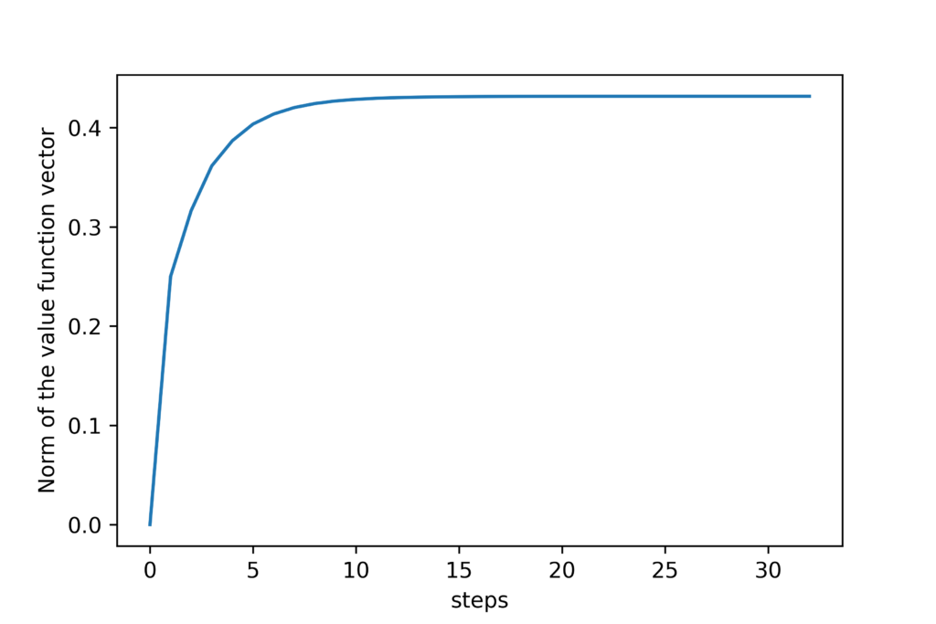
We stop the iteration if the previously explained convergence criterion is satisfied. For visualization purposes, we track the two norm of the vector (6) by using the list convergenceTrack.

We plot the results by using these code lines:

# visualize the state values
def grid_print(valueFunction,reshapeDim):
    ax = sns.heatmap(valueFunction.reshape(4,4),
                     annot=True, square=True,
                     cbar=False, cmap='Blues',
                     xticklabels=False, yticklabels=False)
    plt.savefig('valueFunctionGrid.png',dpi=600)
    plt.show()
    
grid_print(valueFunctionVector,4)

plt.plot(convergenceTrack)
plt.xlabel('steps')
plt.ylabel('Norm of the value function vector')
plt.savefig('convergence.png',dpi=600)
plt.show()

We plot the computed value functions in Fig. 4.

The number in every field represents the computed value function. We can observe that in the terminal states, the function values are zero. Furthermore, we can observe that the function values decrease as we are further away from the goal state. The figure below shows the convergence of the algorithm.

Required Previous Knowledge

Motivation

Test Example

Brief Summary of the Value Function

Iterative Policy Evaluation Algorithm

Python Implementation of the Iterative Policy Evaluation Algorithm

admin

You might also like

3D surface plot of functions in MATLAB using the function fsurf()

Analytically Solve Beam Bending Equation – The Equation of the Elastic Curve of a Cantilever Beam

Solve Optimization Problems in C/C++ by Using NLopt Library