Analytically Solve Beam Bending Equation – The Equation of the Elastic Curve of a Cantilever Beam – Fusion of Engineering, Control, Coding, Machine Learning, and Science

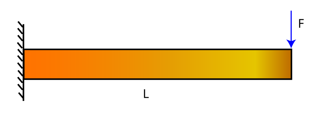
In this lecture, we will learn how to solve an equation of the elastic curve of a cantilever beam. This equation is also known as the beam equation. This equation describes the deflection of the cantilever beam under the action of external forces. The Youtube video accompanying this post is given below.

Problem: Consider the cantilever beam of length $L$ , with the force $F$ acting at its end. Assume that the modulus of elasticity $E$ of the material is known. Also, assume that the moment of inertia $I$ is also known. Define and solve the equation of the elastic curve.

Solution: The first step is to derive a bending-moment diagram. The bending moment diagram is constructed by forming an equilibrium equation for the beam segment shown in the figure below. We perform an imaginary cut at distance $x$ from the beam end.

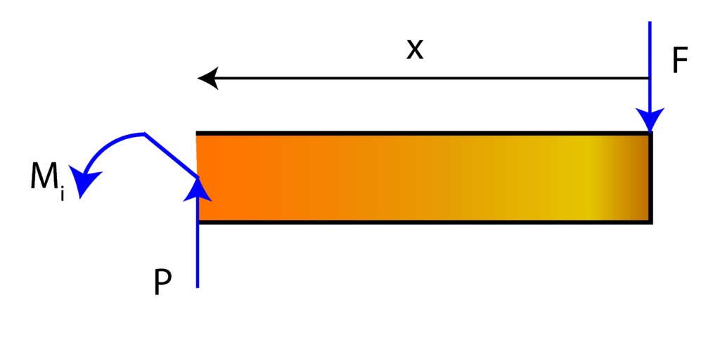
Figure 2: Forces and moments acting at the beam segment.

The force $P$ is an internal force, and moment $M_{i}$ is an internal moment acting at the cross-section. The moment equilibrium equation for a point located at the cross-section has the following form

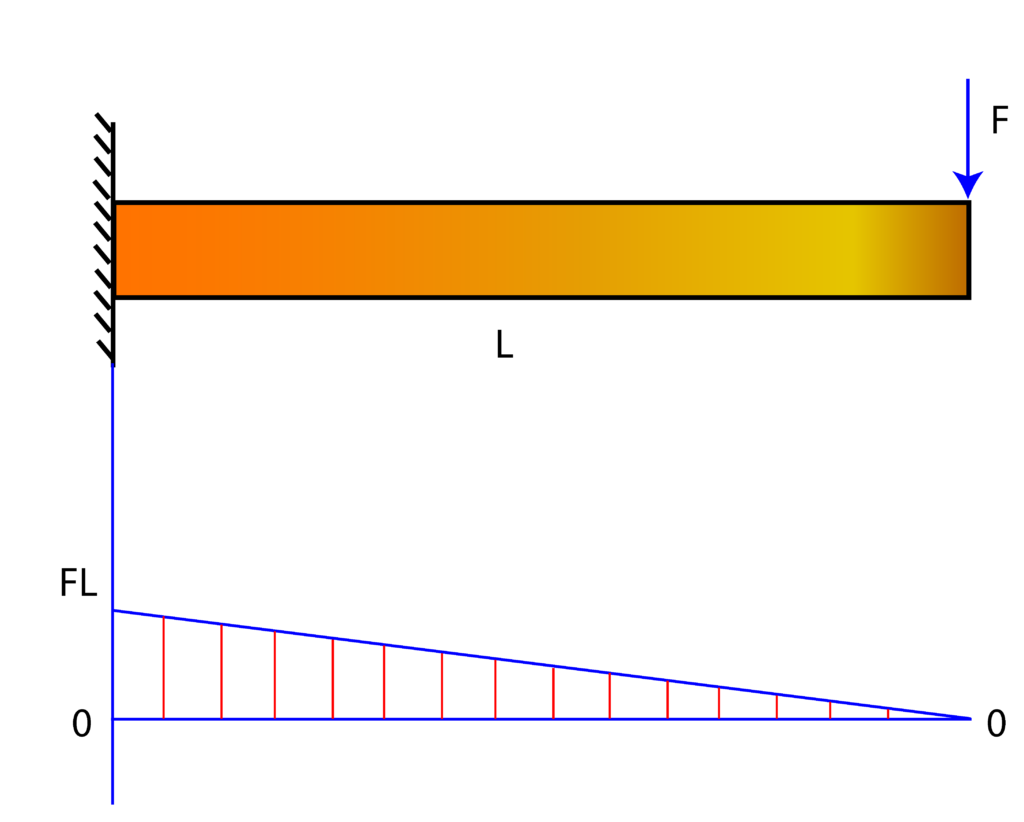
(1) $\begin{align*}-F\cdot x +M_{i}(x)=0 \\M_{i}(x)=F x \end{align*}$

The bending-moment diagram is shown in the figure below.

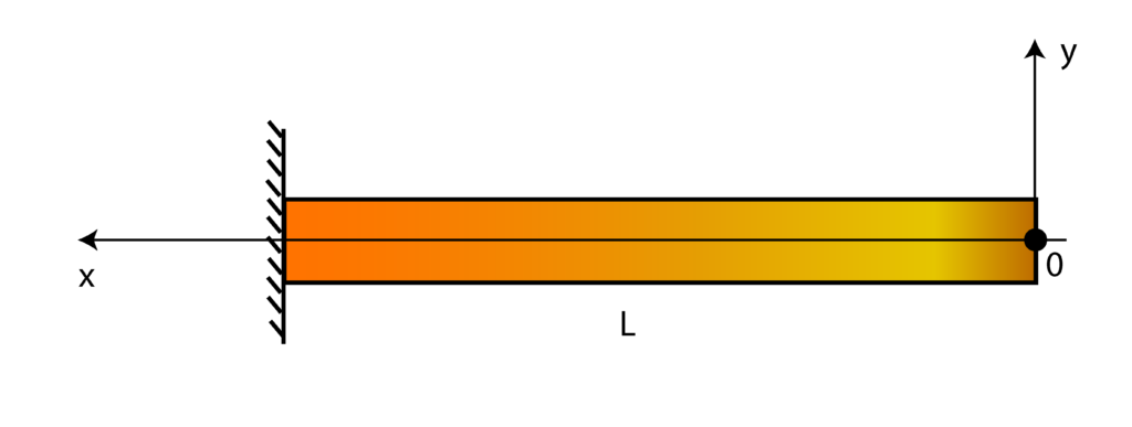
The next step is to choose the location of the coordinate system for defining the equation of the elastic curve.. We select the coordinate system location such that its $x$ -axis and center match the direction of the $x$ -axis and center in Fig. 2. This is done for convenience since the moment equation (1) will not be changed in the assigned coordinate system. The coordinate system is shown in the figure below.

Figure 4: Coordinate system location for defining the equation of the elastic curve.

The governing equation of the elastic curve has the following form

(2) $\begin{align*}EI \frac{d^{2}y}{dx^{2}}=-M_{i}(x)\end{align*}$

It should be emphasized that in (2), there is an extra minus sign compared to some textbooks. However, once the moment is substituted in (2), the final form of the equation will be identical to the equations in other textbooks. This is because of our sign convention for the internal moments in the cross-section shown in Fig. (2).

Substituting (1) in (2), we obtain the final equation of the elastic curve:

(3) $\begin{align*} EI \frac{d^{2}y}{dx^{2}}=- F x \end{align*}$

The last equation can be written as follows

(4) $\begin{align*}EI \;\; d\Big( \frac{dy}{dx} \Big) = - F x \;\;dx\end{align*}$

Now integrating the last equation, we obtain

(5) $\begin{align*}EI \;\; \frac{dy}{dx} = -F\frac{x^2}{2}+C_{1}\end{align*}$

where $C_{1}$ is the constant that we need to determine from boundary conditions. The first-derivative $\frac{dy}{dx}$ quantifies the slope of the elastic curve. Since the cantilever is firmly attached to the wall, the slope for $x=L$ will be zero. That is, the first boundary condition is

(6) $\begin{align*}\frac{dy}{dx}(x=L)=0\end{align*}$

By combining (5) and (6), we obtain

(7) $\begin{align*}EI \cdot 0 = -F\frac{L^2}{2}+C_{1}\end{align*}$

That is,

(8) $\begin{align*}C_{1}= F\frac{L^2}{2} \end{align*}$

By substituting (8) in (5), we obtain

(9) $\begin{align*} EI \;\; \frac{dy}{dx} = -F\frac{x^2}{2}+ F\frac{L^2}{2} \end{align*}$

The last equation can be written as follows

(10) $\begin{align*} EI \;\; dy =\Big( -F\frac{x^2}{2}+ F\frac{L^2}{2} \Big)\;\; dx\end{align*}$

By integrating this equation, we obtain

(11) $\begin{align*}EI \;\; y = -F\frac{x^3}{6} + F\frac{L^2}{2} x+C_{2}\end{align*}$

We find the constant $C_{2}$ from another boundary condition. Namely, when $x=L$ , we have the deformation $y=0$ , since the beam is firmly attached to the wall. We have

(12) $\begin{align*}y(x=L)=0\end{align*}$

By combining (11), and (12), we obtain

(13) $\begin{align*}0 =-F\frac{L^3}{6}+F\frac{L^3}{2}+C_{2}\\C_{2}=FL^3\big(\frac{1}{6} - \frac{1}{2}\big) \\C_{2}= FL^3 \frac{1-3}{6}\\ C_{2}= -FL^3 \frac{1}{3}\\ \end{align*}$