Introduction to MATLAB Control System Toolbox – Defining Models and Computing Responses – Fusion of Engineering, Control, Coding, Machine Learning, and Science

In this post, we provide a brief tutorial on MATLAB Control System Toolbox. The YouTube video accompanying this post is given below.

Consider the following mass-spring-damper system

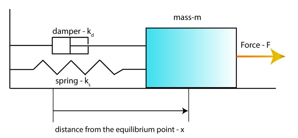
Using second Newton’s law, we can obtain a differential equation describing the motion of the mass-spring-damper system under the action of the force $F$ . The procedure for deriving the differential equation is explained here. The differential equation has the following form

(1) $\begin{align*}m\ddot{x} + k_{d}\dot{x} + k_{s}x=F\end{align*}$

where $x$ is the distance from the equilibrium point, $\dot{x}$ and $\ddot{x}$ are the first and second derivatives of $x$ , $k_{d}$ is the damper constant, $k_{s}$ is the spring constant, and $F$ is the applied force.

Let us now derive the transfer function of the system. By applying the Laplace operator and by ignoring the initial conditions, we obtain the following equation

(2) $\begin{align*}ms^2X(s) +k_{d}sX(s)+k_{s}X(s)=F(s)\end{align*}$

where $s$ is the complex variable, and $X(s)$ is the Laplace transform of $x(t)$ . From (2), we obtain

(3) $\begin{align*}W(s)=\frac{X(s)}{F(s)}=\frac{1}{ms^{2}+k_{d}s+k_{s}}\end{align*}$

where $W(s)$ is the transfer function. Let us now derive the state-space model. First, we introduce the state-space variables

(4) $\begin{align*}x_{1}=x \\x_{2}=\dot{x}\end{align*}$

Using these state-space variables, from (1), we obtain

(5) $\begin{align*}\underbrace{\begin{bmatrix}\dot{x}_{1} \\ \dot{x}_{2} \end{bmatrix}}_{\dot{\mathbf{x}}} = \underbrace{\begin{bmatrix} 0 & 1\\ -\frac{k_{s}}{m} & -\frac{k_{d}}{m} \end{bmatrix}}_{A} \underbrace{\begin{bmatrix}x_{1} \\ x_{2} \end{bmatrix}}_{x}+\underbrace{\begin{bmatrix} 0 \\ \frac{1}{m}\end{bmatrix}}_{B}\underbrace{F}_{u} \end{align*}$

and assuming that the position $x$ is observed, the output equation takes the following form

(6) $\begin{align*}y=\underbrace{\begin{bmatrix} 1 & 0 \end{bmatrix}}_{C}\underbrace{\begin{bmatrix} x_{1} \\ x_{2} \end{bmatrix}}_{\mathbf{x}}+\underbrace{0}_{D}\cdot\underbrace{F}_{u}\end{align*}$

In the sequel, we will explain how to compute step and impulse responses of the system using MATLAB Control System Toolbox. Also, we will explain how to compute the response to arbitrary inputs or initial conditions.

First, we define the model parameters, and define transfer function and state-space system representation. This is done using the following code lines that are self-explanatory.

m=10 
kd=1
ks=10

%% transfer function represenation

num=[1];
den=[m kd ks];

W=tf(num,den)

%% state-space system representation 

A=[0 1; -ks/m -kd/m];
B=[0; 1/m];
C=[1 0];
D=0;
sysSS=ss(A,B,C,D)

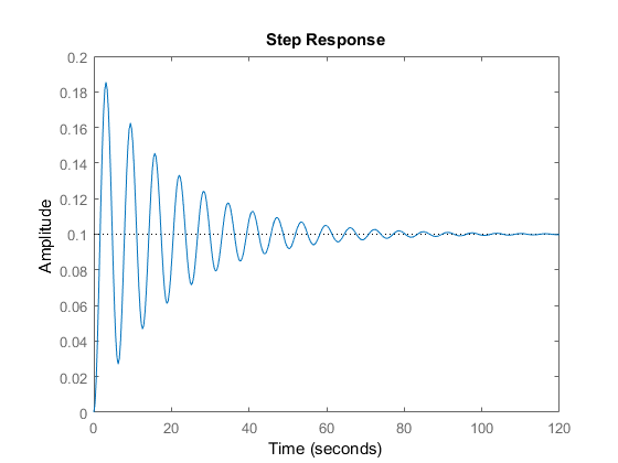
The system step response can be computed in two ways. The following code lines explain this.

%% step response 
% to get the plot window just exectute step(W) or step(sysSS) without
% specifying the output parameters

[step1,timeStep1]=step(W)
[step2,timeStep2]=step(sysSS)

The step-response graph is shown below.

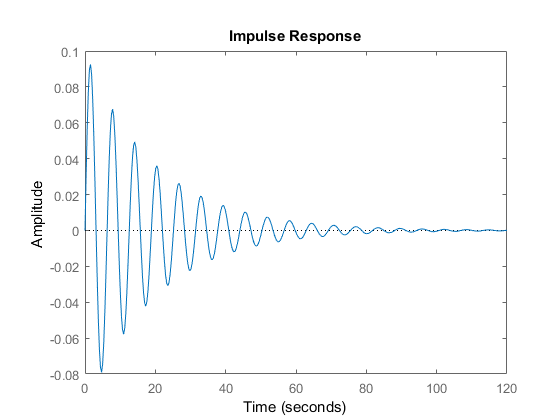
The impulse response can be computes as follows.

%% impulse response

[impulse1,timeImpulese1]=impulse(W)
[impulse2,timeImpulese2]=impulse(sysSS)

The impulse response graph is shown below.

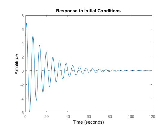
Next, we compute system response for zero inputs and for non-zero initial condition. To the best of our knowledge, this can only be done for the state-space system description (the MATLAB function “initial” does not accept transfer-function system description). The following code lines can be used to compute the system initial condition response.

%% initial condition response 
% define the initial condition
X0=[5;5];

[initial2,timeInitial2]=initial(sysSS,X0)

The initial condition response is shown in the figure below.

Finally, we explain how to compute the system response for arbitrary initial conditions and inputs. The following code lines can be used to perform this task.

%% response to an arbitrary signal and initial condition

X0_lsim=[-0.1,-0.1];
timeSignal=0:0.01:100;
signal=sin(0.5*(timeSignal))+2*ones(size(timeSignal));
[signalResponse, timeSignal1]=lsim(sysSS,signal,timeSignal,X0_lsim)

The results are shown in figure below.

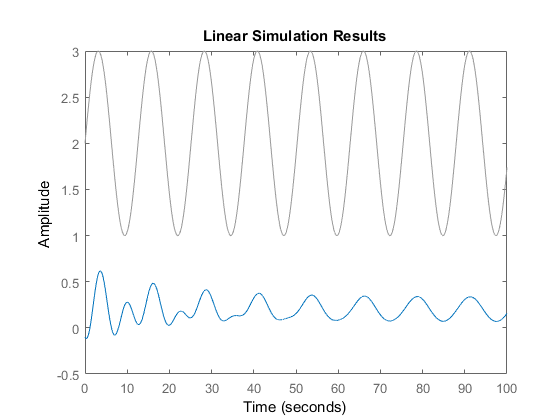
System response to control inputs and non-zero initial conditions.

The gray line in the above figure respresents the control inputs. The blue line represents the system response. By analyzing the shape of the blue line, we can observe that after initial transient reponse, lasting approximately until 40 seconds, the response of the system becomes a sinusoildal signal.

admin

You might also like

COMSOL Tutorial: Thin-Plate Deformation-Introducing Damping

Ways to Support This Channel

Interface (LM393) Encoder with Arduino and Measure the Angle and Angular Velocity