Compute and Simulate Linear Quadratic Regulator (LQR) in MATLAB for Set Point Tracking – Fusion of Engineering, Control, Coding, Machine Learning, and Science

In this post, we provide a brief introduction to Linear Quadratic Regulator (LQR) for set point control. Furthermore, we explain how to compute and simulate the LQR algorithm in MATLAB. The main motivation for developing this lecture comes from the fact that most application-oriented tutorials available online are focusing on the simplified case in which the set point is a zero state (equilibrium point). However, less attention has been dedicated to the problem of regulating the system state to non-zero set points (desired states). The purpose of this lecture and the accompanying YouTube video is to explain how to compute and simulate a general form of the LQR algorithm that works for arbitrary set points. The YouTube video accompanying this post is given below. The GitHub page with all the codes is given here.

The LQR algorithm is arguably one of the simplest optimal control algorithms. Good books for learning optimal control are:

1.) Kwakernaak, H., & Sivan, R. (1972). Linear optimal control systems (Vol. 1, p. 608). New York: Wiley-Interscience.
2.) Lewis, F. L., Vrabie, D., & Syrmos, V. L. (2012). Optimal Control. John Wiley & Sons.
3.) Anderson, B. D., & Moore, J. B. (2007). Optimal Control: Linear Quadratic Methods. Courier Corporation.

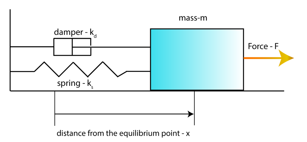
To explain the basic principles and ideas of the LQR algorithm, we use an example of a mass-spring-damper system that is introduced in our previous post, which can be found here. The sketch of the system is shown in the figure below

Figure 1: Sketch of the mass-spring-damper system.

First, we introduce the state-space variables

(1) $\begin{align*}x_{1}=x \\x_{2}=\dot{x}\end{align*}$

where $\dot{x}=\frac{dx}{dt}$ . Then, by using these state-space variables and by using the differential equation describing the system dynamics (see our previous post), we obtain the state-space model

(2) $\begin{align*}\underbrace{\begin{bmatrix}\dot{x}_{1} \\ \dot{x}_{2} \end{bmatrix}}_{\dot{\mathbf{x}}} &= \underbrace{\begin{bmatrix} 0 & 1\\ -\frac{k_{s}}{m} & -\frac{k_{d}}{m} \end{bmatrix}}_{A} \underbrace{\begin{bmatrix}x_{1} \\ x_{2} \end{bmatrix}}_{x}+\underbrace{\begin{bmatrix} 0 \\ \frac{1}{m}\end{bmatrix}}_{B}\underbrace{F}_{u} \\\dot{\mathbf{x}}& =A\mathbf{x}+B\mathbf{u} \end{align*}$

Since in this post, we are considering state feedback, the output equation is not relevant. However, for completeness, we will write the output equation

(3) $\begin{align*}y=\underbrace{\begin{bmatrix} 1 & 0 \end{bmatrix}}_{C}\underbrace{\begin{bmatrix} x_{1} \\ x_{2} \end{bmatrix}}_{\mathbf{x}}+\underbrace{0}_{D}\cdot\underbrace{F}_{u}\end{align*}$

In this particular post and lecture, we assume that the full state information is available at every time instant. That is, we assume that both $x_{1}$ and $x_{2}$ are available. Everything presented in this lecture can be generalized for the case in which only position $x_{1}$ is observed.

The goal of the set point regulation is to steer the system to the desired state (desired set point) $\mathbf{x}_{D}$ , starting from some non-zero initial state (that is in the general case different from $\mathbf{x}_{D}$ ) and under a possible action of external disturbances.

In this post, we will use the terms “desired state” and “desired set point” interchangeably. The first step is to determine the control input $\mathbf{u}_{d}$ that will produce the desired state $\mathbf{x}_{D}$ in the steady-state. Since $\mathbf{x}_{D}$ is constant, by substituting $\mathbf{x}$ by $\mathbf{x}_{D}$ , and $\mathbf{u}$ by $\mathbf{u}_{D}$ in (2), we obtain the following equation

(4) $\begin{align*}0= A\mathbf{x}_{D}+B\mathbf{u}_{D}\end{align*}$

where $\dot{\mathbf{x}}_{D}=0$ since $\mathbf{x}_{D}$ is a constant steady-state. Assuming that the matrix $B$ has full column rank, from (4), we have that the desired control input $\mathbf{u}_{D}$ , producing the desired steady-state $\mathbf{x}_{D}$ , is given by

(5) $\begin{align*} \mathbf{u}_{D} = - (B^{T} B)^{-1} B^{T} A\mathbf{x}_{D} \end{align*}$

In principle, we can control the system by applying the constant control input $\mathbf{u}_{D}$ and by waiting for the system to settle down in the desired steady-state $\mathbf{x}_{D}$ . However, there are several issues with this type of control that can be exaggerated for undamped systems. Namely, the system might exhibit a large overshoot during its transient response, or oscillatory behavior. These phenomena can compromise system safety or performance. Furthermore, the system might be subjected to external disturbances that can seriously deteriorate the control accuracy and performance. These facts motivate the development of the set point feedback control algorithm. The idea is to improve the transient system response and disturbance rejection using a feedback control algorithm.

To develop the control algorithm, we introduce the error variables as follows

(6) $\begin{align*}\tilde{\mathbf{x}}=\mathbf{x}-\mathbf{x}_{D},\;\; => \;\; \mathbf{x} = \tilde{\mathbf{x}} + \mathbf{x}_{D} \\ \tilde{\mathbf{u}}=\mathbf{u}-\mathbf{u}_{D},\;\; => \;\; \mathbf{u} = \tilde{\mathbf{u}} + \mathbf{u}_{D} \end{align*}$

By differentiating these expressions and by substituting (6) in (2), we obtain

(7) $\begin{align*}\dot{\mathbf{x}}= \dot{\tilde{\mathbf{x}}}+ \dot{\mathbf{x}}_{D}=A(\tilde{\mathbf{x}}+ \mathbf{x}_{D}) +B(\tilde{\mathbf{u}}+\mathbf{u}_{D}) \end{align*}$

Here it should be kept in mind that since $\mathbf{x}_{D}$ is constant, we have $\dot{ \mathbf{x}}_{D}=0$ . By substituting this in (7), we obtain

(8) $\begin{align*} \dot{\tilde{\mathbf{x}}} = A\tilde{\mathbf{x}}+B\tilde{\mathbf{u}}+A\mathbf{x}_{D}+B\mathbf{u}_{D}\end{align*}$

On the other hand, by substituting (4) in (8), we obtain

(9) $\begin{align*} \dot{\tilde{\mathbf{x}}} = A\tilde{\mathbf{x}}+B\tilde{\mathbf{u}} \end{align*}$

Having this form of dynamics, we can straightforwardly apply the LQR algorithm that is derived under the assumption of zero desired state. The LQR algorithm optimizes the following cost function

(10) $\begin{align*}J(\tilde{\mathbf{u}})=\int_{t=0}^{t=\infty}\Big(\mathbf{\tilde{x}}^{T}Q \mathbf{\tilde{x}} + \mathbf{\tilde{u}}^{T}R \mathbf{\tilde{u}} +2 \mathbf{\tilde{x}}^{T}N \mathbf{\tilde{u}} \Big) \; dt\end{align*}$

where $Q$ , $R$ , and $N$ are the weighting matrices. The cost function is constrained by the system dynamics (9). The weighting matrices should be selected by the user and they need to satisfy a few assumptions (as well as the system matrices for the solution of the LQR problem to exist, however, in order not to blur the main ideas of this post with unnecessary mathematical perplexities, we will not discuss further these conditions). The matrix $Q$ penalizes the control error, and generally speaking, larger values of $Q$ will increase the speed of the system response. However, the trade-off is that more control energy will be spent to steer the system to the zero state. On the other hand, the matrix $R$ penalizes the control energy. Larger values of $R$ will generally minimize the control energy, however, at the expense of reducing the system’s response speed. In our simulations, we will assume that $N$ is a zero matrix. Furthermore, to simplify the control design, we will assume that the weighting matrices are diagonal. That is, we assume that

(11) $\begin{align*}Q=q\cdot I, \;\; R=r \cdot I\end{align*}$

where $I$ is an identity matrix, and $q>0$ and $r>0$ are positive real numbers. The solution that optimizes the cost function (10) is the feedback control law of the following form

(12) $\begin{align*}\tilde{\mathbf{u}}=-K\tilde{\mathbf{x}}\end{align*}$

where the matrix $K$ is defined by

(13) $\begin{align*}K=R^{-1}(B^{T}S+N^{T})\end{align*}$

where $S$ is the solution of the algebraic matrix Riccati equation:

(14) $\begin{align*}A^{T}S+SA-(SB+N)R^{-1}(B^{T}S+N^{T})+Q=0\end{align*}$

Fortunately, we do not need to write our own code for solving the Riccati equation. We will use the MATLAB function lqr() to compute the control matrix $K$ . By substituting (12) in (9), we obtain the closed-loop system

(15) $\begin{align*}\dot{\tilde{\mathbf{x}}}=(A-BK)\tilde{\mathbf{x}}\end{align*}$

The LQR control algorithm will make the matrix $A-BK$ asymptotically stable (all the eigenvalues of A-BK are in the left-half of the complex plane). This means that the set-point state error $\tilde{\mathbf{x}}$ will asymptotically approach zero. That is, in the steady-state, the system state $\mathbf{x}$ will become $\mathbf{x}_{D}$ . From (15) , we have

(16) $\begin{align*}\dot{\mathbf{x}}=(A-BK)\mathbf{x}- (A-BK) \mathbf{x}_{D}\end{align*}$

The equation (16) can be used to simulate the closed loop system.

Taking into account the error variables (6), we can write the feedback control (12), as follows

(17) $\begin{align*}\mathbf{u}=\mathbf{u}_{D}-K(\mathbf{x}-\mathbf{x}_{D}) \end{align*}$

We now proceed with defining the system in MATLAB and with simulations.

First, using the procedure explained in our previous post, we define the system state-space representation:

clear, pack, clc

% mass
m=10 
% damping 
kd=5
% spring constant
ks=10


%% state-space system representation 

A=[0 1; -ks/m -kd/m];
B=[0; 1/m];
C=[1 0];
D=0;
sysSS=ss(A,B,C,D)

Then, we define the desired state, and we compute the steady-state control input using (5).

%% define the desired state 
xd=[3;0];


%% compute ud

ud=-inv(B'*B)*B'*A*xd

The desired state is $x_{1}=3$ and $x_{2}=0$ . Next, for the computed $\mathbf{u}_{D}$ , we simulate the system response. We apply this constant control input and observe the state trajectory. The following code lines are used to simulate the system response.

%% simulate the system response for the computed ud

% set initial condition
x0=1*randn(2,1);

%final simulation time 

tFinal=30;

time_total=0:0.1:tFinal;
input_ud=ud*ones(size(time_total));

[output_ud_only,time_ud_only,state_ud_only] = lsim(sysSS,input_ud,time_total,x0); 

figure(1)
plot(time_total,state_ud_only(:,1),'k')
hold on 
plot(time_total,state_ud_only(:,2),'r')
xlabel('Time [s]')
ylabel('Position and velocity')
legend('Position','Velocity')
grid

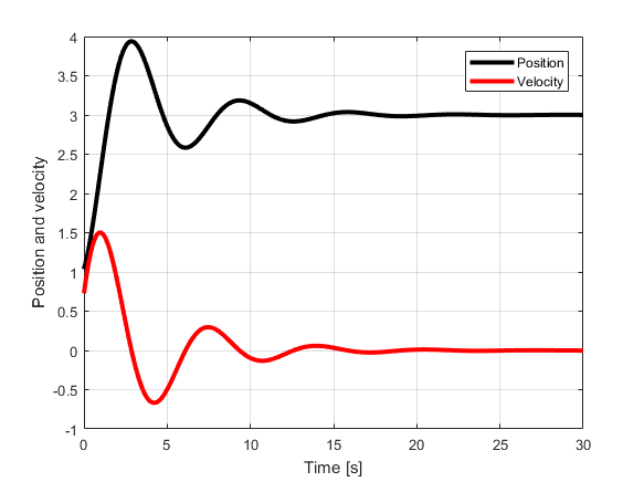
The figure below shows the simulated state trajectories. The position ( $x_{1}$ ) and velocity ( $x_{2}$ ) start from an arbitrary initial condition that is set by the user. We observe that approximately after 25 seconds the position settles at 3 and velocity settles at 0. These are actually desired steady-states that are set by the user when computing $\mathbf{u}_{D}$ . We see that the constant control input is able to steer the system’s state to the desired steady-state. However, we can also observe large overshoots. The LQR algorithm will have significant advantages over this control approach, if it is able to reduce the overshoots and to increase the control convergence speed.

Figure 2: Simulated state trajectories for the constant steady-state input.

The next goal is to simulate the LQR algorithm. We compute the control matrix $K$ using the MATLAB function lqr(). To compute the control matrix, we defined the weighting matrices $Q$ and $R$ as diagonal matrices. Finally, we have simulated the closed loop system. We have used the equation (16) to simulate the closed loop system. The code is given below.

%% simulate the LQR algorithm 

Q= 10*eye(2,2);
R= 0.1;
N= zeros(2,1);

[K,S,e] = lqr(sysSS,Q,R,N);

% compute the eigenvalues of the closed loop system 
eig(A-B*K)

% eigenvalues of the open-loop system 
eig(A)

%simulate the closed loop system 
% closed loop matrix 
Acl= A-B*K;

Bcl=-Acl;
C=[1 0];
D=0;
sysSSClosedLoop=ss(Acl,Bcl,C,D)

closed_loop_input=[xd(1)*ones(size(time_total));
                    xd(2)*ones(size(time_total))];


[output_closed_loop,time_closed_loop,state_closed_loop] = lsim(sysSSClosedLoop,closed_loop_input,time_total,x0); 




figure(2)
plot(time_total,state_ud_only(:,1),'k')
hold on 
plot(time_total,state_ud_only(:,2),'r')
xlabel('Time [s]')
ylabel('Position and velocity')
plot(time_closed_loop,state_closed_loop(:,1),'m')
hold on 
plot(time_closed_loop,state_closed_loop(:,2),'b')
legend('Position-Constant Input ','Velocity-Constant Input','Position-Closed Loop ','Velocity-Closed Loop')
grid

Here, we compare the state trajectories of the closed loop system (LQR algorithm) with the state trajectories of the system for the constant steady-state input. This is done to investigate the performance gain obtained by using the LQR algorithm.

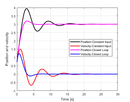
Figure 3: Comparison of the state trajectories of the closed-loop system and the system with constant steady-state input.

From Fig. 3., we can clearly observe the advantages of the LQR algorithm. We can observe that the overshoot is decreased and that the convergence is much faster compared to the system that is controlled using the steady-state control input. Also, the eigenvalues of the matrix A are

-0.2500 + 0.9682i
-0.2500 – 0.9682i

And the eigenvalues of the closed-loop matrix A-BK are

-0.7208 + 0.9458i
-0.7208 – 0.9458i

Since the real parts of the eigenvalues of the closed-loop matrix are almost 3 times further left in the complex plane compared to the eigenvalues of the open-loop system, we can see that the closed-loop system has much more favorable poles from the stability point of view compared to the poles of the open-loop system.

admin

You might also like

Simulation of Ordinary Differential Equations (ODEs) with Time-varying Coefficients and Time-varying Inputs in MATLAB

March 16, 2021: Scary wind-induced oscillations of the Verrazzano-Narrows Bridge

Ray Tracing with COMSOL – First Part