Ray Tracing with COMSOL – First Part – Fusion of Engineering, Control, Coding, Machine Learning, and Science

In this post and in the accompanying video, we will learn how to set up and perform a basic ray tracing task with COMSOL Multiphysics. In the second part, we will learn how to generate spot diagrams and in the third part, we will learn how to generate aberration plots. Note: First read this post and then watch the video.

For simplicity and presentation clarity we will analyze ray propagation through a thin lens. Everything learned in this post can be generalized to more complex systems. Consider a sketch shown in the following figure.

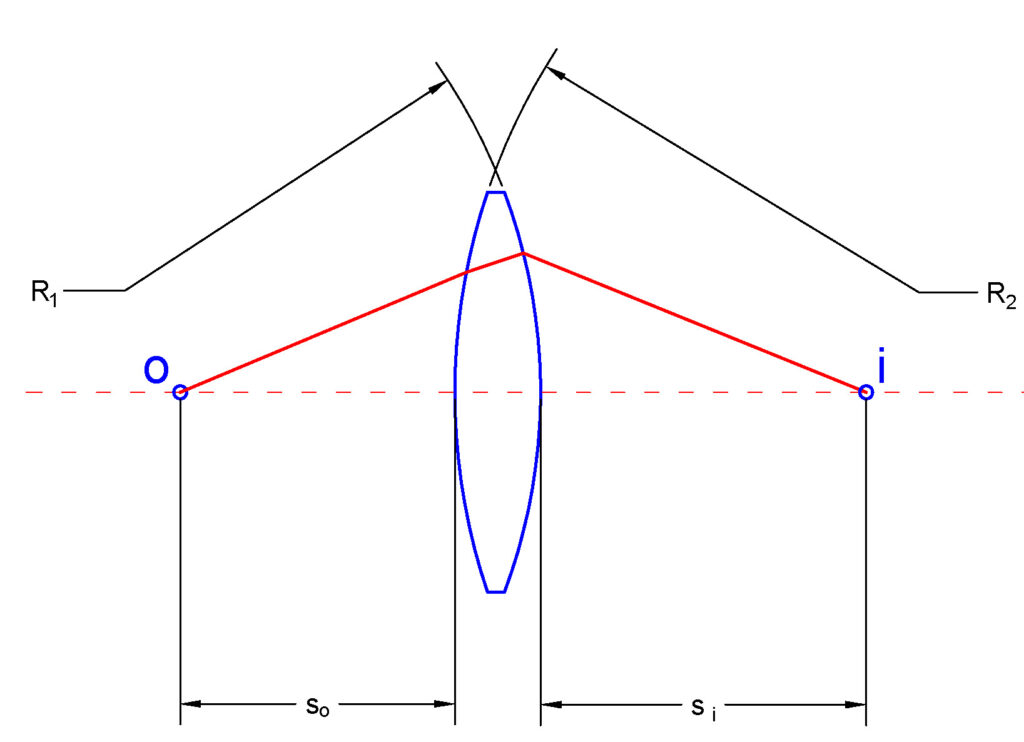
Figure 1: Ray propagation through a thin lens. Note: lens thickness is a exaggerated.

We consider a thin spherical lens with lens surface diameters of $R_{1}$ and $R_{2}$ . The lens is surrounded by the medium with the refraction index of $n_{m}=1$ . The ray starting from the point $O$ (object point) is propagated to the point $i$ (image point). The distance of the point $O$ to the front vertex of the lens is $s_{O}$ and the distance from the image point $i$ to the back vertex of the lens is $s_{i}$ . Notice that since our assumption is that lens is thin, $s_{O}$ is approximately equal to the distance from the center of the lens on the optical axis to the object point. Similarly, $s_{i}$ is approximately equal to the distance from the center of the lens on the optical axis to the image point.

Under the paraxial ray assumption (as well as under some other assumptions, see for example Eugene Hecht’s book : “Optics”), the positions $s_{O}$ and $s_{i}$ are related via the following formula:

(1) $\begin{align*}\frac{1}{s_{O}}+\frac{1}{s_{i}}=(n_{l}-1)(\frac{1}{R_{1}}+\frac{1}{R_{2}})\end{align*}$

where $n_{l}$ is the refraction index of the lens. The last equation is the famous Thin Lens Equation or Lensmaker’s formula. Using this formula we can predict the distance of the image point, knowing the distance of the object point. When the object point is moved to the focal point of the lens, then the image point is far away from the lens, that is, the image point tends to infinity. In this case, we have

(2) $\begin{align*} \lim_{s_{i}->\infty} s_{O}=f\end{align*}$

where $f$ is the focal point. In that case from (1), we have

(3) $\begin{align*}\frac{1}{s_{0}}+\frac{1}{\infty}=(n_{l}-1)(\frac{1}{R_{1}}+\frac{1}{R_{2}})\end{align*}$

or using the fact that in this case $s_{O}=f$ , we have

(4) $\begin{align*}\frac{1}{f}=(n_{l}-1)(\frac{1}{R_{1}}+\frac{1}{R_{2}})\end{align*}$

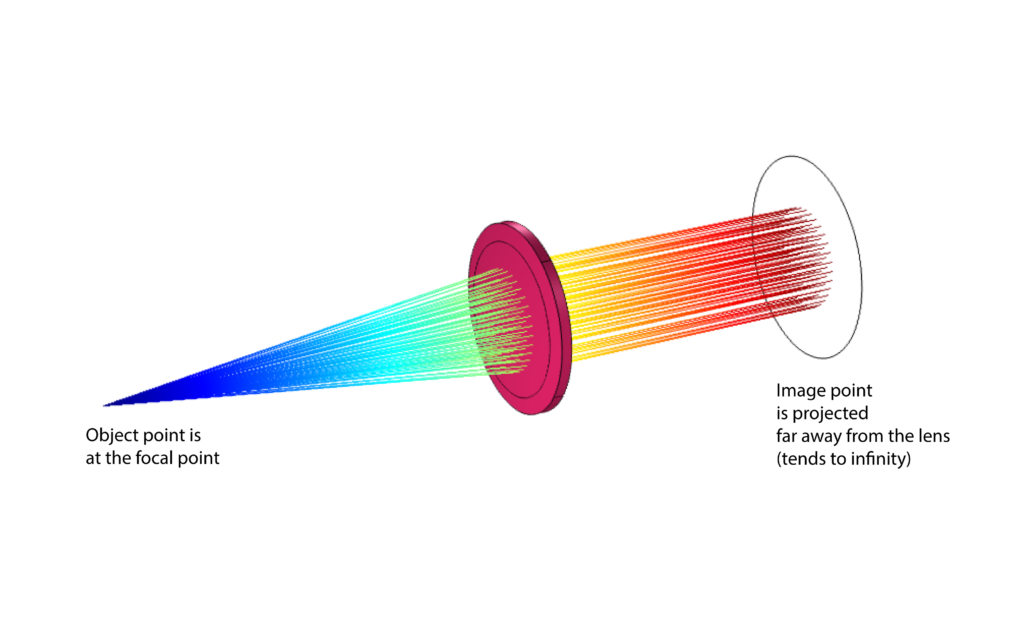
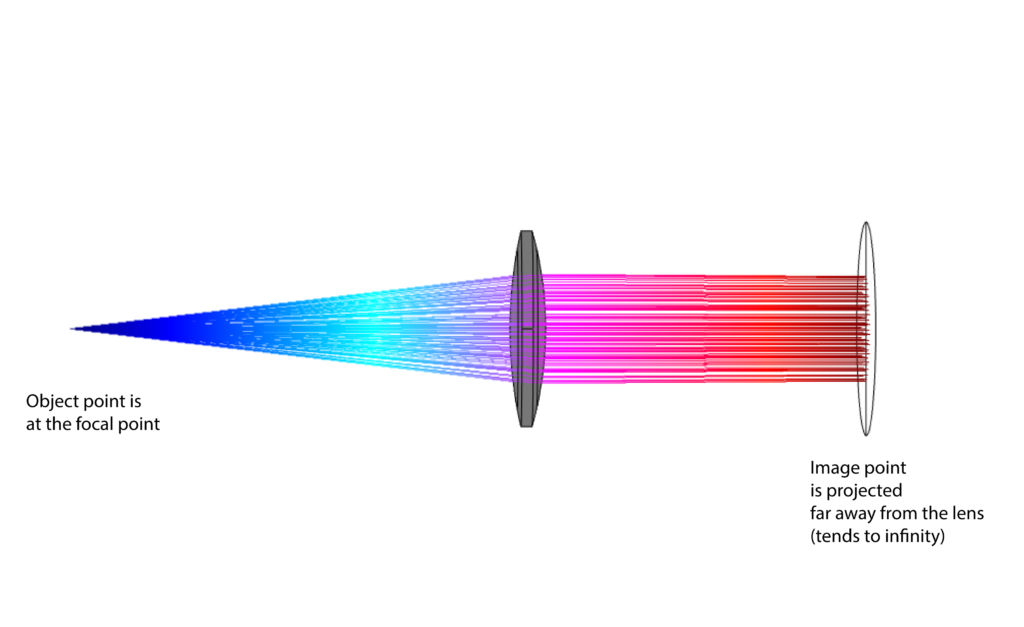
The equation (4) is useful since it enables to estimate the focal point location. This is important for verifying COMSOL simulations and for comparing simulations with a priori knowledge derived from the physical laws. This situation corresponds to the following ray-tracing images computed using COMSOL Multiphysics.

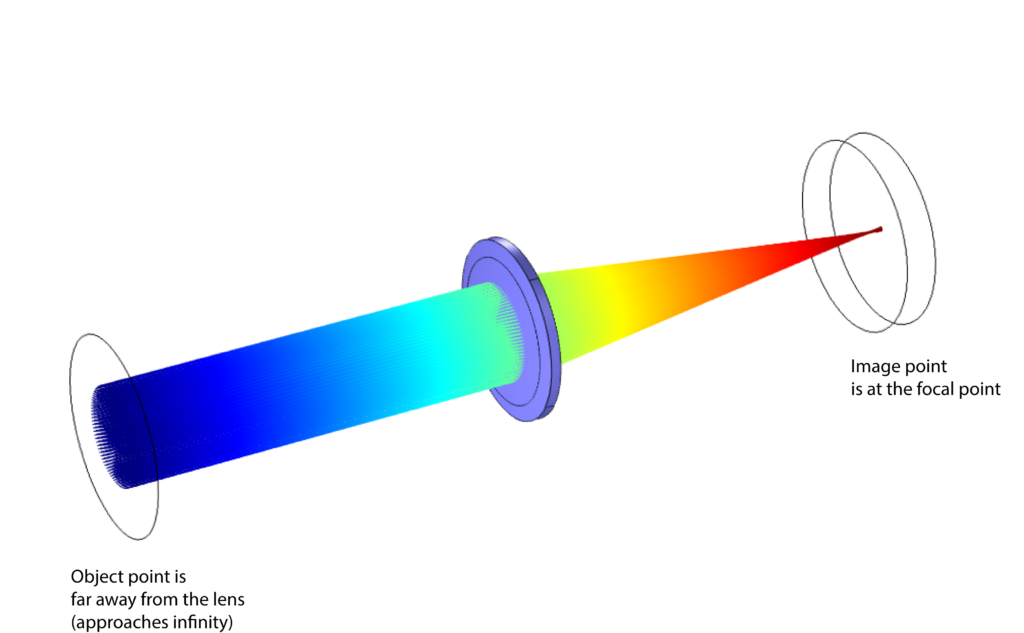
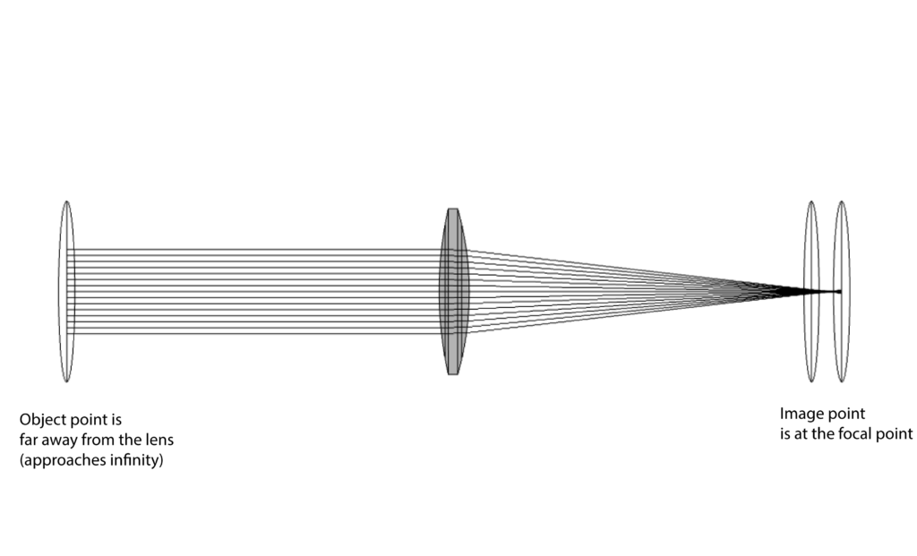
*Figure 3: Ray tracing diagram generated using COMSOL when the object point is placed at the focus point.*

*Figure 4: Ray tracing diagram generated using COMSOL when the object point is placed at the focus point.*

On the other hand, when the object point is far away from the lens (tends to infinity) then the image object is at the focal point. This means that the rays coming from the object far away from the lens tend to be parallel to the optical axis and they are focused at the focal point. That is,

(5) $\begin{align*}\lim_{s_{o}->\infty} s_{i}=f\end{align*}$

In that case from (1), we have

(6) $\begin{align*}\frac{1}{\infty}+\frac{1}{s_{i}}=(n_{l}-1)(\frac{1}{R_{1}}+\frac{1}{R_{2}})\end{align*}$

or using the fact that in this case $s_{i}=f$ , we have

(7) $\begin{align*}\frac{1}{f}=(n_{l}-1)(\frac{1}{R_{1}}+\frac{1}{R_{2}})\end{align*}$

Comparing the last equation with (4), we conclude that for a thin lens, the lengths of the focal points for the two cases are the same. Ray tracing for the case when the object point is far away from the lens is visualized by the following figures that are generated using COMSOL Multiphysics.

*Figure 5: Ray tracing diagram generated using COMSOL when the object point is far away from the lens (approaches infinity).* *The image point is then at the focal point.*

*Figure 6: Ray tracing diagram generated using COMSOL when the object point is far away from the lens (approaches* infinity). The image point is then at the focal point.

By expressing the focal distance either from (4) or (7), we obtain

(8) $\begin{align*}f=\frac{R_{1}R_{2}}{(n_{l}-1)(R_{2}-R_{1})}\end{align*}$

Following the convention rules, when substituting values for $R_{1}$ and $R_{2}$ in the previous formula, $R_{1}$ should be taken with a positive sign and $R_{2}$ should be taken with a negative sign.

In our COMSOL simulations, we have $R_{1}=125 [mm]$ and $R_{2}=-100 [mm]$ . For lens material, we use silica glass with the refraction index of $1.45$ . The computed focal lens distance is $f=123.46$ . All other modeling steps are explained in the video.