Control Systems Lecture: Simulation of linear ordinary differential equations using Python and state-space modeling – Fusion of Engineering, Control, Coding, Machine Learning, and Science

In this post, we provide an introduction to state-space models and explain how to simulate linear ordinary differential equations (ODEs) using the Python programming language. State-space modeling and numerical simulations are demonstrated using an example of a mass-spring system. A detailed video accompanying this post is given below.

Mass-spring systems are widely used to model the dynamics of actuators and other electromechanical devices. A basic sketch of a mass-spring system is given in Figure 1 below.

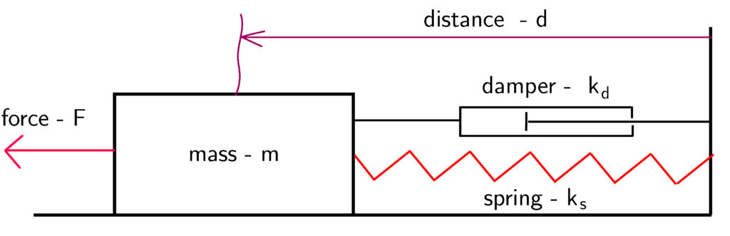
Figure 1: A sketch of a mass-spring system.

An object of mass $m$ is attached to a spring and a damper. The spring constant is $k_{s}$ and the damper constant is $k_{d}$ . The purpose of the damper is to damp the mechanical oscillations. Let us assume that the object is at its equilibrium position. If an external force $F$ is acting on the system, then the object will move in the direction of the force. How do we mathematically describe this motion?
To mathematically describe the oscillations, we first need to construct a free-body diagram. The free-body diagram is given in Figure 2 below.

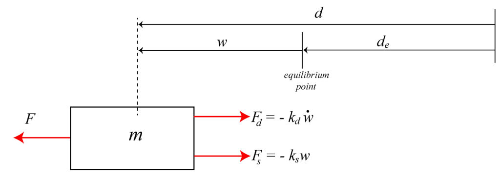
Figure 2: The free-body diagram of the mass-spring system.

In the equilibrium point, the spring is in its neutral position, and consequently, it does not exert a force on the object. In Fig.2, $d_{e}$ is the distance from the wall to the equilibrium point. The variable $w$ is used to describe the distance of the object from the equilibrium point. The spring force $F_{s}$ is given by the following equation

(1) $\begin{align*}F_{s}=-k_{s}w\end{align*}$

That is, the spring force is proportional to the displacement from the equilibrium point. The sign is opposite from the sign of the variable $w$ . If $w$ is positive, the spring is expanded and the spring force tends to bring the object to its equilibrium position. The damper force $F_{d}$ is given by the following equation:

(2) $\begin{align*} F_{d}=-k_{d}\dot{w} \end{align*}$

The damper force is proportional to the object’s velocity that is denoted by $\dot{w}$ and the sign is opposite from the sign of the velocity. That is, the damper force sign is opposite from the direction of the movement. In Figure 2, we assumed that the direction of the movement is in the direction of the $w$ -axis. The dynamics of the object is governed by Newton’s second law:

(3) $\begin{align*}m\vec{a}=\sum_{i=1}^{n}\vec{F}_{i}\end{align*}$

where $\vec{a}$ is the acceleration vector and $F_{i}$ is the $i$ -th force acting on the system. Projecting this equation onto the $w$ axis, and using the equations (1) and (2) we obtain the following equation:

(4) $\begin{align*}m\ddot{w}=F-k_{d}\dot{w}-k_{s}w\end{align*}$

The last equation can be written as follows:

(5) $\begin{align*}m\ddot{w} +k_{d}\dot{w}+k_{s}w =F\end{align*}$

This equation mathematically describes the effect of the force $F$ onto the movement of the object. This is a second-order, linear ODE. This equation is linear since the variable $w$ and its derivatives $\dot{w}$ and $\ddot{w}$ appear as linear functions. The equation’s order is determined by the highest derivative, which in our case is equal to $2$ . The general solution of this equation is defined as follows:

(6) $\begin{align*}w=w\big(t,w(0),\dot{w}(0),F(t)\big)\end{align*}$

where $w(0)$ and $\dot{w}(0)$ are the initial position and velocity, respectively, $t$ is time, and $F(t)$ is a force as a function of time. Our goal is not to find an exact analytical form of the solution given by equation (6). Instead, our goal is to numerically solve the equation (5).

To numerically solve this equation, we will write it as a system of first-order ODEs. More generally, an $n$ -th order ODE can be written as a system of $n$ first-order ODEs. This system actually defines a state-space model of the system.

To define a state-space model, we first need to introduce state variables. The state variables are denoted by $x_{1}$ and $x_{2}$ . We define the state variables as follows:

(7) $\begin{align*}x_{1}&=w \\ x_{2}&=\dot{w} \label{x2} \label{stateVariables}\end{align*}$

By differentiating the last two equations, we obtain:

(8) $\begin{align*} \dot{x}_{1}&=\dot{w}=x_{2} \\ \dot{x}_{2}&=\ddot{w}=-\frac{k_{d}}{m}\dot{w}-\frac{k_{s}}{m}w+\frac{1}{m}F= -\frac{k_{d}}{m}x_{2}-\frac{k_{s}}{m}x_{1}+\frac{1}{m}F \label{x2d} \label{differentiationStateSpace}\end{align*}$

where we have used the equation (5) to express $\dot{x}_{2}$ as a function of $x_{1}$ and $x_{2}$ . The last equation can be written in a vector form:

(9) $\begin{align*}\underbrace{\begin{bmatrix}\dot{x}_{1} \\ \dot{x}_{2} \end{bmatrix}}_{\dot{\mathbf{x}}}= \underbrace{\begin{bmatrix}0 & 1 \\ -\frac{k_{s}}{m} & -\frac{k_{d}}{m} \end{bmatrix}}_{A}\underbrace{ \begin{bmatrix} x_{1} \\ x_{2} \end{bmatrix}}_{\mathbf{x}} + \underbrace{\begin{bmatrix} 0 \\ \frac{1}{m} \end{bmatrix}}_{B}\underbrace{F}_{u}\end{align*}$

(10) $\begin{align*}\dot{\mathbf{x}}=A\mathbf{x}+Bu \end{align*}$

where $\mathbf{x}$ is the state vector, $u=F$ is the control input, and $A$ and $B$ are system matrices defined in equation (9). With the state equation (10) we need to associate an output equation. The output equation maps the state vector into the output vector (in our case it will be a scalar). A system output is a system variable or a function of system variables whose dynamical behavior we want to track. We usually measure the system output using sensors. In our case, the output equation has the following form:

(11) $\begin{align*}y=\underbrace{\begin{bmatrix}1 & 0 \end{bmatrix}}_{C} \mathbf{x} \end{align*}$

That is, we are measuring the state variable $x_{1}$ that corresponds to the displacement from the equilibrium position, denoted by $w$ . The state-space and output equations are usually written next to each other:

(12) $\begin{align*}\dot{\mathbf{x}}&=A\mathbf{x} + B\mathbf{u}\\ \mathbf{y}&=C\mathbf{x} \\ \end{align*}$

The main question is how to simulate the system (12) for given initial conditions $\mathb{x}_{1}(0)$ and $\mathb{x}_{2}(0)$ . The first approach is to use a forward Euler method. Namely, using the forward Euler method, we can approximate the derivative $\dot{\mathbf{x}}$ as follows:

(13) $\begin{align*}\dot{\mathbf{x}}\approx \frac{\mathbf{x}_{k+1}- \mathbf{x}_{k}}{h}\end{align*}$

where $h$ is a discretization time constant (usually a small real number), $k$ denotes a discrete-time instant $kh$ , $k=0,1,2,3,\ldots$ , $\mathbf{x}_{k}$ is an approximation of the state vector at the time instant $kh$ , that is an approximation of $\mathbf{x}(kh)$ . Subsituting the equation (13) in the state-space model (12), we obtain

(14) $\begin{align*}& \mathbf{x}_{k+1}=\underbrace{\big(I + hA \big)}_{A_{df}} \mathbf{x}_{k} + \underbrace{hB}_{B_{df}} u_{k} \\& \mathbf{y}_{k} = C\mathbf{x}_{k}\end{align*}$

where $\mathbf{y}_{k}$ and $u_{k}$ are defined in the same manner as the discretized state variable $\mathbf{x}_{k}$ . From the equation (14) we see that we can obtain the discretized state sequence $\mathbf{x}_{1}, \mathbf{x}_{2}, \mathbf{x}_{3},\ldots$ by simply propagating the equation

(15) $\begin{align*} \mathbf{x}_{k+1}=A_{df}\mathbf{x}_{k}+B_{df}u_{k}\end{align*}$

from the initial condition $\mathbf{x}_{0}$ and using the control input sequence $u_{0}, u_{1}, u_{2},\ldots$ . However, this approach might produce numerical instabilities of the discretized state vector $\mathbf{x}_{k}$ (the state vector might diverge to infinity). To avoid this problem, it is preferable to discretize the system using the backward Euler method. The backward Euler method discretizes the state sequence as follows:

(16) $\begin{align*} \dot{\mathbf{x}}\approx \frac{\mathbf{x}_{k}- \mathbf{x}_{k-1}}{h} \end{align*}$

Subsituting the equation (16) in the state equation of the state-space model (12), we obtain:

(17) $\begin{align*}\big(I -hA \big)\mathbf{x}_{k}= \mathbf{x}_{k-1}+hBu_{k}\end{align*}$

From this equation, we obtain:

(18) $\begin{align*} \mathbf{x}_{k}=A_{db}\mathbf{x}_{k-1}+B_{db}u_{k}\end{align*}$

where

(19) $\begin{align*} A_{db} = \big(I-hA\big)^{-1}, \;\; B_{db}= h \big(I - hA\big)^{-1}B\end{align*}$

Starting from the initial condition $\mathbf{x}_{0}$ and using the control input sequence $u_{1},u_{2},u_{3},\ldots$ , we can generate the discretized state sequence $\mathbf{x}_{1}, \mathbf{x}_{2}, \mathbf{x}_{3}, \ldots$ , by propagating the equation (18). Once the state sequence is generated, we can easily generate the output sequence by using the equation $y_{k}=C\mathbf{x}_{k}$ . We use this method to discretize the state-space model.

The Python code for discretizing the state-space model is given below.

import numpy as np
import matplotlib.pyplot as plt

# define the continuous-time system matrices

A=np.matrix([[0, 1],[- 0.1, -0.05]])
B=np.matrix([[0],[1]])
C=np.matrix([[1, 0]])
#define an initial state for simulation
x0=np.random.rand(2,1)

#define the number of time-samples used for the simulation and the sampling time for the discretization
time=300
sampling=0.5

#define an input sequence for the simulation
#input_seq=np.random.rand(time,1)
input_seq=np.ones(time)
#plt.plot(input_sequence)


# the following function simulates the state-space model using the backward Euler method
# the input parameters are:
#    -- A,B,C              - continuous time system matrices 
#    -- initial_state      - the initial state of the system 
#    -- time_steps         - the total number of simulation time steps 
#    -- sampling_perios    - the sampling period for the backward Euler discretization 
# this function returns the state sequence and the output sequence
# they are stored in the vectors Xd and Yd respectively
def simulate(A,B,C,initial_state,input_sequence, time_steps,sampling_period):
    from numpy.linalg import inv
    I=np.identity(A.shape[0]) # this is an identity matrix
    Ad=inv(I-sampling_period*A)
    Bd=Ad*sampling_period*B
    Xd=np.zeros(shape=(A.shape[0],time_steps+1))
    Yd=np.zeros(shape=(C.shape[0],time_steps+1))
    
    for i in range(0,time_steps):
       if i==0:
           Xd[:,[i]]=initial_state
           Yd[:,[i]]=C*initial_state
           x=Ad*initial_state+Bd*input_sequence[i]
       else:
           Xd[:,[i]]=x
           Yd[:,[i]]=C*x
           x=Ad*x+Bd*input_sequence[i]
    Xd[:,[-1]]=x
    Yd[:,[-1]]=C*x
    return Xd, Yd
    
state,output=simulate(A,B,C,x0,input_seq, time ,sampling)    


plt.plot(output[0,:])
plt.xlabel('Discrete time instant-k')
plt.ylabel('Position- d')
plt.title('System step response')

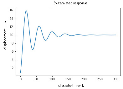
A few comments are in order. The code lines 6-8 are used to define an arbitrary mass-spring system. The code line 10 is used to define an initial condition. The code line 13 is used to define the total number of discrete-time steps. The code line 14 defines the discretization time constant $h$ . The code line 18 defines a control input sequence. The control input sequence is equal to $1$ at every time sample. This is a so-called step input sequence, and the corresponding output is called the step response of the system. The code lines 30-49 define a function for discretizing the state-space model. The code lines 51-57 are used to generate the system output and to plot it. The result is given in Figure 3 below.

admin

You might also like

State-Space Modeling of Double Mass-Spring-Damper System with Python Modeling

Correct Explanation of State Observers for State Estimation of State-Space Models with Python Simulations

Control Systems Lecture: Laplace Transform