Control Systems Lecture: DC motor state-space modeling and MATLAB’s Control System Toolbox simulations – Fusion of Engineering, Control, Coding, Machine Learning, and Science

In this post, we explain how to model a DC motor and to simulate control input and disturbance responses of such a motor using MATLAB’s Control Systems Toolbox. We obtain a state-space model of the system. This model is used in other lectures to demonstrate basic control principles and algorithms. This post is based on Chapter 4 of “Feedback Control of Dynamic Systems (third edition)” by Franklin, Power, and Emami-Naeini. A YouTube video accompanying this post is given below.

Here we will not discuss the working principle of DC motors. We assume that the reader has a basic understanding of the main physical laws governing the behavior of DC motors. For a nice introduction to DC motors, see for example this webpage. Figure 1(a) shows a basic electrical circuit of a DC motor. Figure 1(b) shows a free body diagram of the rotor.

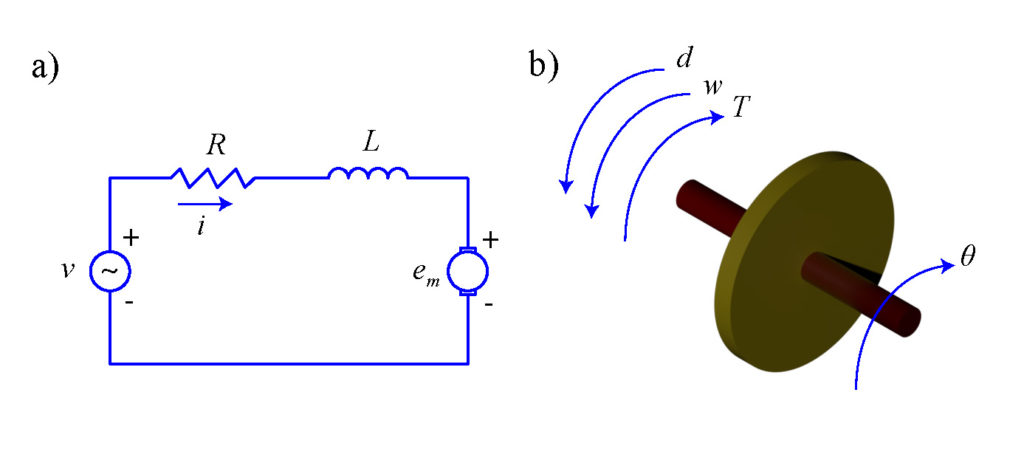
Figure 1: (a) a basic electrical circuit of a DC motor and (b) a free body diagram of the motor rotor.

A basic equation governing the mechanical dynamics of the motor is

(1) $\begin{align*}J\ddot{\theta}=T-w-d\end{align*}$

where $J$ is the rotor inertia, $\theta$ is the angle of rotation of the output shaft, $T$ is a mechanical torque developed in the motor rotor, $w$ is a disturbance torque, and $d$ is a damping torque. From the motor law, we have:

(2) $\begin{align*}T=K_{T}i\end{align*}$

where $i$ is the armature current and $K_{T}$ is a torque constant. That is, the generated torque is proportional to the armature current. On the other hand, the damping torque can be expressed as follows:

(3) $\begin{align*}d=b\dot{\theta}\end{align*}$

where $b$ is a damping coefficient. By substituting the last two equations in equation (1) describing the motor mechanical dynamics, we obtain the following equation:

(4) $\begin{align*} J\ddot{\theta}+ b\dot{\theta}=K_{T}i-w \end{align*}$

The armature current has its own dynamics. From Figure 1(a), we can write:

(5) $\begin{align*}L\dot{i}+Ri=v-e_{m}\end{align*}$

where $e_{m}$ is the back electromotive force given by the following equation:

(6) $\begin{align*}e_{m}=K_{e}\dot{\theta}\end{align*}$

By substituting the equation (6) in the equation (5), we obtain:

(7) $\begin{align*} L\dot{i}+Ri=v-K_{e}\dot{\theta} \end{align*}$

The equations (4) and (7) govern the dynamics of the DC motor, and for clarity we write them next to each other:

(8) $\begin{align*} J\ddot{\theta}+ b\dot{\theta}=K_{T}i-w \end{align*}$

(9) $\begin{align*} L\dot{i}+Ri=v-K_{e}\dot{\theta} \end{align*}$

The voltage $v$ is an external voltage used to control the motor.

State-space model

Our main goal is to write the equations (8) and (9) in a state-space form:

(10) $\begin{align*}& \dot{\mathbf{x}}=A\mathbf{x}+Bu+Wd \\& y=C\mathbf{x}\end{align*}$

where $\mathbf{x}=\begin{bmatrix} x_{1} & x_{2} & x_{3} \end{bmatrix}^{T}$ is a state vector, $u$ is the control input vector, $y$ is the system output (a scalar), and $A,B,C$ and $W$ are the system matrices.

We introduce the state-space variables, control input variables, and the output variable as follows:

(11) $\begin{align*}x_{1}=\theta \notag \\x_{2}= \dot{\theta} \\x_{3}=i \\y=x_{2} \\u=v \end{align*}$

A few comments are in order. We need 3 state-space variables because the overall system order is equal to 3. How do we determine the overall system order? The overall system order is equal to the sum of the orders of two differential equations. The order of the first differential equation (8) (the highest derivative apearing the differential equation) is 2, and the order of the second differential equation (9) is 1. The output of the system is our choice. However, this choice should be in accordance with our practical ability to observe (measure) the output variable. In our case, the output variable is the angular velocity $\dot{\theta}$ . The control input $u$ is equal to the variable that is used to control the system. In our case, it is the external voltage $v$ . From the equations (8), (9), and (11), we have

(12) $\begin{align*}&\dot{x}_{1}=x_{2} \notag \\&\dot{x}_{2}=\ddot{\theta}=\frac{K_{T}}{J}x_{3}-\frac{1}{J}d- \frac{b}{J}x_{2} \notag \\ &\dot{x}_{3}=\dot{i}=\frac{1}{L}u-\frac{R}{L}x_{3}-\frac{K_{e}}{L}x_{2} \notag \\&y=\begin{bmatrix}0 & 1 & 0 \end{bmatrix}\begin{bmatrix} x_{1}\\ x_{2} \\ x_{3} \end{bmatrix}\end{align*}$

These equations can be written in a state-space form:

(13) $\begin{align*}& \underbrace{\begin{bmatrix}\dot{x}_{1} \\ \dot{x}_{2} \\ \dot{x}_{3} \end{bmatrix}}_{\dot{\mathbf{x}}}= \underbrace{\begin{bmatrix} 0 & 1 & 0 \\ 0 & -\frac{b}{J} & \frac{K_{T}}{J} \\ 0 & -\frac{K_{e}}{L} & -\frac{R}{L} \end{bmatrix}}_{A} \underbrace{\begin{bmatrix} x_{1} \\ x_{2} \\ x_{3} \end{bmatrix}}_{\mathbf{x}}+\underbrace{\begin{bmatrix} 0 \\ 0 \\ \frac{1}{L} \end{bmatrix}}_{B} u + \underbrace{\begin{bmatrix} 0 \\ -\frac{1}{J} \\ 0 \end{bmatrix}}_{W}d \\& y=\underbrace{\begin{bmatrix} 0 & 1 & 0 \end{bmatrix}}_{C}\underbrace{\begin{bmatrix}x_{1} \\ x_{2} \\ x_{3} \end{bmatrix}}_{\mathbf{x}}\end{align*}$

In the sequel, we present the MATLAB code for simulating the state-space model. First we define the model.

clear,pack,clc

% define the constants
J=0.1
b=0.5
Kt=1
L=1
R=5
Ke=1
L=1

% define the system matrices
A=[0 1 0; 0 -b/J Kt/J; 0 -Ke/L -R/L]
B=[0; 0; 1/L]
W=[0; -1/J; 0]
C=[0 1 0]

% combine the control input and disturbance matrices in a single matrix
Btotal=[B W]

% define the state-space model
sys = ss(A,Btotal,C,[])

% discretization constant
dt = 0.01;
% final simulation time 
Tfinal= 5;
% discretized time
discretization_time = 0:dt:Tfinal;

A few comments are in order. The code lines 13-16 are used to define the system matrices. The code line 19 is used to augment the control input and disturbance matrices. The code line 22 is used to define the state-space model. The MATLAB function ss() takes as input parameters the system matrices, and it produces the state-space model. The code lines 24-29 are used to define the discretization constant, final simulation time, and the vector (“discretization_time “) containing the discretization time steps.

The next code block is used to generate a step control input signal, and to compute and plot the system step response. The system step response is important for understanding the dynamics of the system. It is generated by actuating the system with a step control input function.

%%%%%%%%%%%%%%%%%%%%%%%%%%%%%%%%%%%%%%%%%%%%%%%%%%%%%%%%%%%%%%%%%%%%%%%%%%%
% system response to the step control input 
%%%%%%%%%%%%%%%%%%%%%%%%%%%%%%%%%%%%%%%%%%%%%%%%%%%%%%%%%%%%%%%%%%%%%%%%%%%

% control input
figure(1)
control_step = ones(size(discretization_time))';
plot(discretization_time,control_step,'LineWidth',2)
xlabel('Time')
ylabel('Control input (voltage)')
title('Control Input Used for Simulation')

% disturbance 
disturbance = zeros(size(discretization_time))';

% control input and disturbance
U_step=[control_step, disturbance];

% simulate the system
Ycontrol_step=lsim(sys,U_step,discretization_time);

% plot the system output 
figure(2)
plot(discretization_time,Ycontrol_step,'LineWidth',2)
xlabel('Time')
ylabel('System output (angular velocity)')
title('System response to the step control input')

The code line 7 is used to generate a step control input signal. The code line 14 is used to generate a zero disturbance signal. That is, we assume that the disturbance torque $w$ is not affecting the system dynamics while computing the step response. The code line 17 is used to augment the control and disturbance control signals (remember that the state-space model is defined for two control input signals). The code line 20 is used to simulate the system. This is achieved using the MATLAB function lsim(). The output of this function is the vector Ycontrol_step which contains the system output defined at the discrete-time samples in vector discretization_time. Other code lines are used to generate the plots. The results are shown in Fig. 2 below.

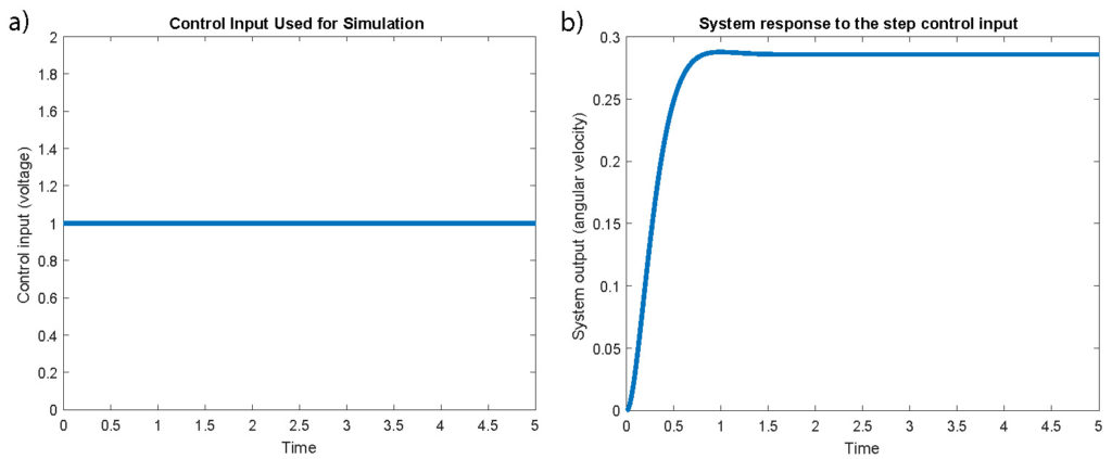
Figure 2: (a) the step control input and (b) the system step response.

From Fig. 1 it follows that the system step response is highly damped. The next code block computes the system response to a sinusoidal control input signal. The code lines are analogous to the code lines in the previous code block.

%%%%%%%%%%%%%%%%%%%%%%%%%%%%%%%%%%%%%%%%%%%%%%%%%%%%%%%%%%%%%%%%%%%%%%%%%%%
% system response to the sinusoidal control input 
%%%%%%%%%%%%%%%%%%%%%%%%%%%%%%%%%%%%%%%%%%%%%%%%%%%%%%%%%%%%%%%%%%%%%%%%%%%

% control input
figure(3)
control_sin = (4+sin(5*discretization_time))';
plot(discretization_time,control_sin,'LineWidth',2)
xlabel('Time')
ylabel('Control input (voltage)')
title('Control Input Used for Simulation')

% disturbance 
disturbance = zeros(size(discretization_time))';

% control input and disturbance
U_sin=[control_sin, disturbance];

% simulate the system
Ycontrol_sin=lsim(sys,U_sin,discretization_time);

% plot the system output 
figure(4)
plot(discretization_time,Ycontrol_sin,'LineWidth',2)
xlabel('Time')
ylabel('System output (angular velocity)')
title('System response to the sinusoidal control input')

Sinusoidal control input and a corresponding response are shown in Fig. 3 below.

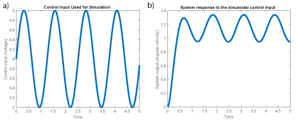
*Figure 3: (a) the sinusoidal control input and (b) the system response.*

From Fig.3 we can observe that the system is able to track the sinusoidal control input signal.

The next code block is used to simulate the system response to non-zero initial conditions. During this simulation, the control and disturbance signals are zero. The initial condition is $\mathbf{x}(0)=\begin{bmatrix} 1 & 1 & 1 \end{bmatrix}^{T}$

%%%%%%%%%%%%%%%%%%%%%%%%%%%%%%%%%%%%%%%%%%%%%%%%%%%%%%%%%%%%%%%%%%%%%%%%%%%
% system response to non zero inital conditions
%%%%%%%%%%%%%%%%%%%%%%%%%%%%%%%%%%%%%%%%%%%%%%%%%%%%%%%%%%%%%%%%%%%%%%%%%%%
X0=[1; 1; 1];
Yinitial=initial(sys,X0,discretization_time);
% plot the system output 
figure(5)
plot(discretization_time,Yinitial,'LineWidth',2)
xlabel('Time')
ylabel('System output (angular velocity)')
title('System response to the initial condition')

The code line 5 is used to compute the system’s initial condition response. The results are given in Fig. 4 below.

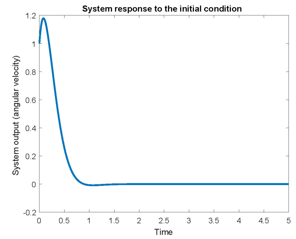
Figure 4: the system’s response to non-zero initial conditions.

We can use Fig. 4 to argue about system stability. Since the response decays to zero, we conclude that the system is “most likely” stable.

State-space model

admin

You might also like

Compute Magnitude and Phase Responses (Frequency Response) of Digital Filters and Discrete-Time Systems in Python

Automatic State-Space Derivation and Simulation of Nonlinear Dynamical Systems in Python with Inverted Pendulum on a Cart Example

Implementation of the Solution of the Linear Quadratic Regulator (LQR) Control Algorithm in C++ by Using the Eigen Matrix Library.