Compute Magnitude and Phase Responses (Frequency Response) of Digital Filters and Discrete-Time Systems in Python – Fusion of Engineering, Control, Coding, Machine Learning, and Science

In this digital signal processing and discrete-time control tutorial, we will learn how to compute the magnitude and phase responses of digital filters and discrete-time systems in Python. The magnitude and phase responses are uniquely called the frequency response of a digital filter. To compute the frequency response, we will use the symbolic Python toolbox called SymPy. SymPy will enable us to symbolically compute the real and imaginary parts of the complex transfer functions. Then, we will transform symbolic expressions into Python functions that will enable us to compute the phase and magnitude responses.

In our previous tutorial given here, we thoroughly explained the concept of the frequency response of digital filters and discrete-time systems. Consequently, before continuing with this tutorial, it is strongly advised to read that tutorial. The YouTube video is given below.

Python Script for Computing the Frequency Response of Digital Filters

The frequency response consists of two responses:

Magnitude response
Phase response

As a test case, we consider the following filter

(1) $\begin{align*}y[n]=\frac{1}{2}\big(x[n]-x[n-1] \big)\end{align*}$

where $y[n]$ is the output sequence and $x[n]$ is the input sequence. To compute the frequency response, we need to derive the transfer function. For that purpose, we apply the Z-transform to (1)

(2) $\begin{align*}\mathcal{Z}\{ y[n] \}=\frac{1}{2}\mathcal{Z}\{ x[n] \}-\frac{1}{2}\mathcal{Z}\{ x[n-1] \}\end{align*}$

Let us introduce this notation for the $Z$ -transform

(3) $\begin{align*}\mathcal{Z}\{ y[n] \}= Y(z) \\\mathcal{Z}\{ x[n] \}=X(z)\end{align*}$

Taking into account that the $Z$ -transform of the delayed signal is given by $\mathcal{Z}\{ x[n-1] \}=z^{-1}X(z)$ , from (2), we have

(4) $\begin{align*}Y(z)=\frac{1}{2}X(z)-\frac{1}{2}z^{-1}X(z)\end{align*}$

(5) $\begin{align*}Y(z)=\frac{z-1}{2z} X(z) \end{align*}$

Consequently, the transfer function is

(6) $\begin{align*}\frac{Y(z)}{X(z)}=H(z)=\frac{z-1}{2z}\end{align*}$

To compute the frequency response, we substitute $z$ with $e^{j\omega}$ , where $\omega$ is the digital frequency. As a result, we obtain the following expression

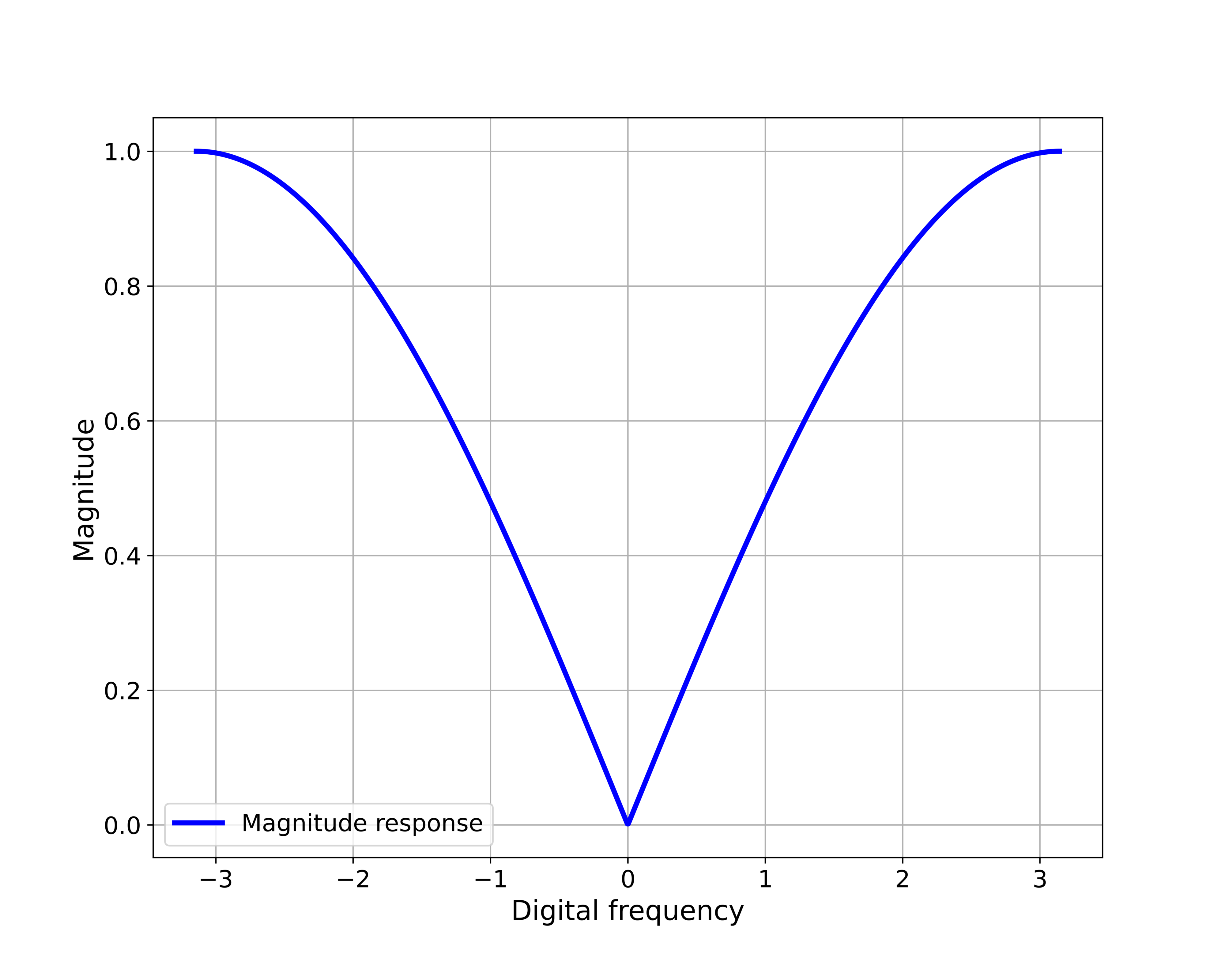
(7) $\begin{align*}H(e^{j\omega})=\frac{e^{j\omega}-1}{2e^{j\omega}}\end{align*}$

In our previous tutorial, given here, we derived the expressions for the magnitude and phase responses that result from the equation (7). The magnitude response is

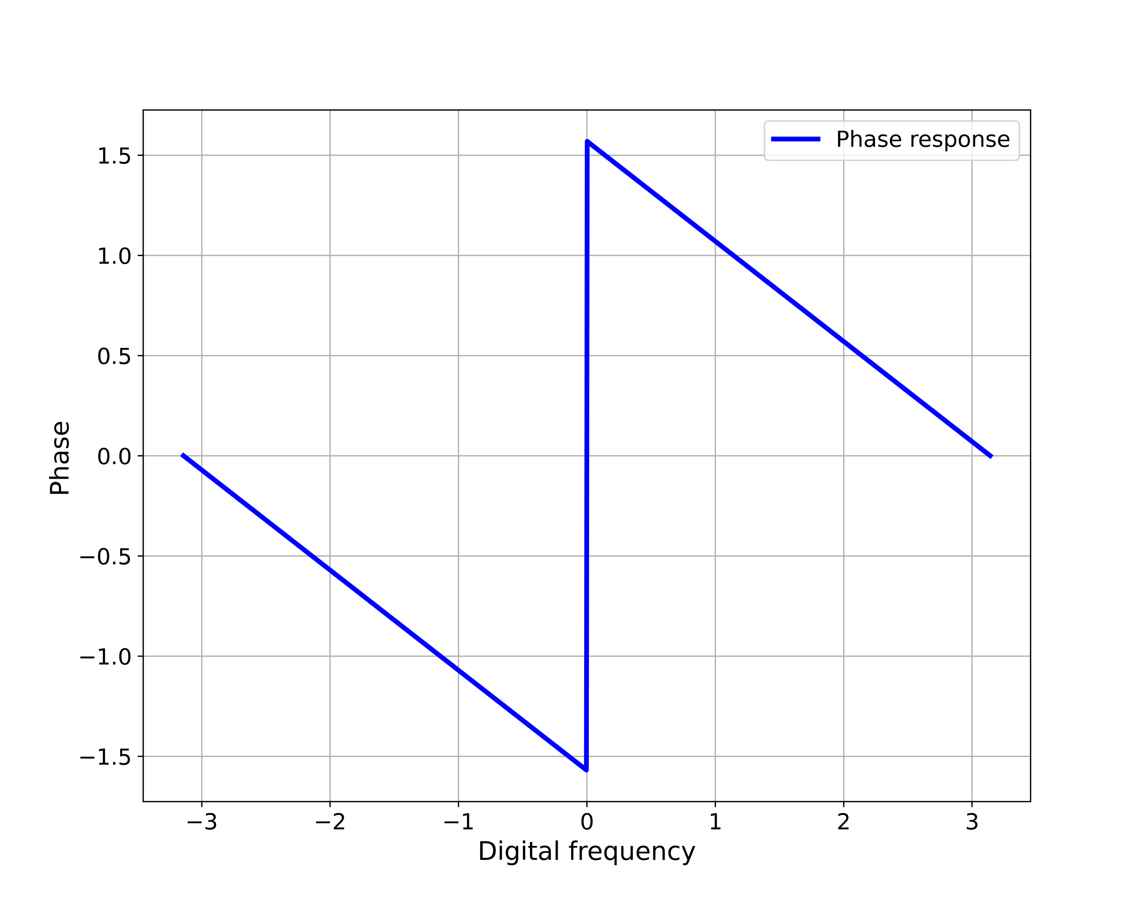
(8) $\begin{align*}M(\theta)=|\sin(\frac{\omega}{2})|\end{align*}$

The phase response is

(9) $\begin{align*}\theta (\omega )&=-\frac{\omega}{2}+\frac{\pi}{2} ,\;\; \text{for} \;\; 0 \le \omega \le \pi \\\theta (\omega )& =-\frac{\omega}{2}-\frac{\pi}{2} ,\;\; \text{for} \;\; -\pi \le \omega \le 0\end{align*}$

These two formulas will be used to double-check the results obtained by using the Python script presented in the sequel.

First, we compute the magnitude and phase responses by using the formulas (8) and (9). The Python script is given below.

import numpy as np
from sympy import *
import matplotlib.pyplot as plt
# symbolic digital frequency
w = Symbol('w', real=True)

# numerical digital frequency
# it should be in the interval from -pi to pi 
omega=np.linspace(-np.pi,np.pi,1000)

# First approach
# This is the manual approach

# vectors to store magnitude and phase
magnitudeFirstApproach=np.abs(np.sin(omega/2))
phaseFirstApproach=np.zeros(len(magnitudeFirstApproach))

# compute the phase
for index in range(len(omega)):
    if (omega[index]>=0):
        phaseFirstApproach[index]=np.pi/2-omega[index]/2
    else:
        phaseFirstApproach[index]=-np.pi/2-omega[index]/2

We simply define the vector of frequencies “omega” and we substitute this vector in (8) and (9). Note that at the beginning of this script, we import the complete SymPy library and we also define a symbolic variable “w”. This symbolic variable denoted the digital frequency $\omega$ .

Next, we use the symbolic approach to compute the frequency response. The idea is to first compute the symbolic expression for (7) and then to compute the symbolic real and imaginary parts. Once the real and imaginary parts are computed, we can automatically create functions for real and imaginary parts. These functions will take the numerical values of the frequency $\omega$ and return the corresponding real and imaginary parts. Once we have these functions, we can compute the phase response. We use a similar approach to compute the magnitude response. We compute the symbolic expression for the magnitude and then, define a function that returns the numerical value of magnitude for the given value of frequency.

The following Python script performs these tasks.

# second approach
# this is the symbolic approach
# freqeuncy response function 
# I is the imaginary unit 
# E is the exponential function
H=(E**(I*w)-1)/(2*E**(I*w))

# extract real and imaginary parts
funcReal=re(H)
funcIm=im(H)

funcRealComp=lambdify(w,funcReal)
funcImagComp=lambdify(w,funcIm)

realParts=funcRealComp(omega)
imagParts=funcImagComp(omega)

phaseSymbolic=np.arctan2(imagParts,realParts)

# check the difference between the two approaches
phaseDiff=np.max(np.abs(phaseSymbolic-phaseFirstApproach))


# compute the magnitude
M=abs(H)
magFun=lambdify(w,M)
magnitudeSymbolic=magFun(omega)
magnitudeDiff=np.max(np.abs(magnitudeFirstApproach-magnitudeSymbolic))

Once we define the symbolic expression for $H$ , we use the SymPy functions “re()” and $im()$ to extract the real and imaginary parts of $H$ . We use the Python function “lambdify()” to create functions out of symbolic expressions. To compute the symbolic expression for the magnitude, we use the SymPy function “abs”. We also compute the difference between the approaches for computing the magnitude and phase responses. The errors given by variables “phaseDiff” and “magnitudeDiff” are very small. This means that the symbolic approach for computing the magnitude and phase calculates almost identical values to the values given by the formulas (8) and (9).

The following Python script is used to generate the graphs that show the magnitude and phase responses.


# plot the results 
plt.figure(figsize=(10,8))
plt.plot(omega,magnitudeFirstApproach,'b',linewidth=7,label='Magnitude response')
plt.xlabel('Digital frequency',fontsize=16)
plt.ylabel('Magnitude',fontsize=16)
plt.legend(fontsize=14)
plt.tick_params(axis='both', which='major', labelsize=14)
plt.grid()
plt.savefig('magnitudeFirst.png',dpi=600)
plt.show()

plt.figure(figsize=(10,8))
plt.plot(omega,phaseFirstApproach,'b',linewidth=7,label='Phase response')
plt.xlabel('Digital frequency',fontsize=16)
plt.ylabel('Phase',fontsize=16)
plt.legend(fontsize=14)
plt.tick_params(axis='both', which='major', labelsize=14)
plt.grid()
plt.savefig('phaseFirst.png',dpi=600)
plt.show()

The graphs generated by this Python script are given below.

Python Script for Computing the Frequency Response of Digital Filters

admin

You might also like

How To Properly Simulate a Stochastic (Random) Linear State-Space Model in Python

Pole Placement With Integral Control Action to Eliminate Steady-State Error (State-Space Control Design)

Clear and Concise Explanation of Fourier Series With Solved Examples and Python code