Symbolic and Automatic Linearization of Nonlinear Systems in Python by Using SymPy Library – Fusion of Engineering, Control, Coding, Machine Learning, and Science

In this Python and control engineering tutorial, we will learn one very important scientific computing technique that can be used to implement classical and advanced control and estimation algorithms. We will learn how to automatize the linearization of nonlinear systems in Python by using Python’s symbolic computation library called SymPy. The method presented in this video tutorial is very important for designing controllers and estimators for high-order nonlinear dynamical systems where it is practically impossible to perform linearization by hand. Before reading this tutorial it is a very good idea to get yourself familiar with the basics of linearization of nonlinear systems. Consequently, we strongly suggest you thoroughly study our tutorial on the linearization of nonlinear systems given here. The YouTube video accompanying this post is given here.

Test Case 1: Linearization of Nonlinear Pendulum Equations

This is our first test case for testing our approach for automatic differentiation and linearization. In our previous tutorial given here, we derived a nonlinear state-space model of a pendulum system. This is the classical system for testing linear and nonlinear control engineering algorithms. The pendulum is shown in the figure below.

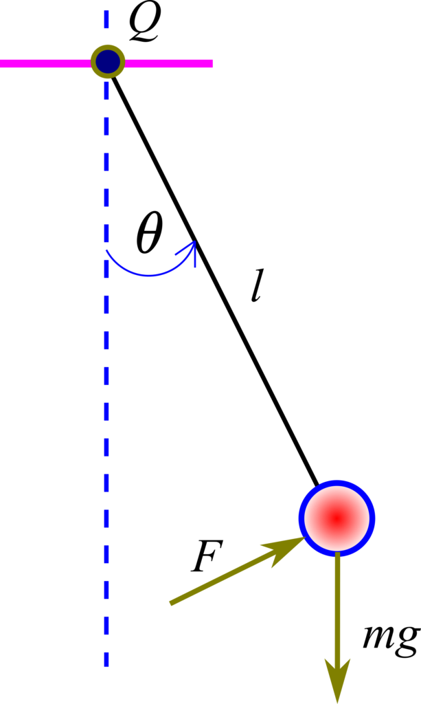
In the figure above, $l$ is the length of the pendulum, $m$ is the mass of the ball, $g$ is the gravitational acceleration constant, $\theta$ is the angle of the pendulum, and $F$ is the control force. By using the state-space variables:

(1) $\begin{align*}x_{1}=\theta\\x_{2}=\dot{\theta}\end{align*}$

where $\dot{\theta}$ is the angular velocity, we obtain the nonlinear pendulum state-space model of the pendulum

(2) $\begin{align*}\begin{bmatrix} \dot{x}_{1} \\ \dot{x}_{2} \end{bmatrix}=\begin{bmatrix}x_{2} \\ -\frac{g}{l}\sin (x_{1}) +\frac{1}{ml}u^{2} \end{bmatrix}\end{align*}$

where $u$ is the control input. To derive this state-space model, we assumed that the control force $F$ is $F=u^{2}$ . Our state space model can be written in the standard form

(3) $\begin{align*}\dot{\mathbf{x}}=\mathbf{f}(\mathbf{x},u)\end{align*}$

where the state vector is

(4) $\begin{align*}\mathbf{x}=\begin{bmatrix} x_{1} \\ x_{2} \end{bmatrix}\end{align*}$

and the vector function $\mathbf{f}(\cdot )$ is defined by

(5) $\begin{align*}\mathbf{f}=\begin{bmatrix}f_{1} \\ f_{2} \end{bmatrix}\end{align*}$

where

(6) $\begin{align*}f_{1}&=x_{2} \\f_{2}&=-\frac{g}{l}\sin(x_{1})+\frac{1}{ml}u^2\end{align*}$

To linearize the state-space model, we need to compute the Jacobian matrices of the nonlinear vector function $\mathbf{f}(\cdot)$ with respect to the state vector $\mathbf{x}$ and the control input $u$ .

The state Jacobian matrix is defined by

(7) $\begin{align*}\frac{\partial \mathbf{f}}{\partial \mathbf{x} } =\begin{bmatrix} \frac{\partial f_{1}}{\partial x_{1}} & \frac{\partial f_{1}}{\partial x_{2}} \\ \frac{\partial f_{2}}{\partial x_{1}} & \frac{\partial f_{2}}{\partial x_{2}} \end{bmatrix}=\begin{bmatrix} 0 & 1\\ -\frac{g}{l}cos(x_{1}) & 0 \end{bmatrix}\end{align*}$

The input Jacobian matrix is defined by

(8) $\begin{align*}\frac{\partial \mathbf{f}}{\partial \mathbf{u} } =\begin{bmatrix} \frac{\partial f_{1}}{\partial u} \\ \frac{\partial f_{2}}{\partial u}\end{bmatrix} =\begin{bmatrix} 0 \\ \frac{2}{ml} u\end{bmatrix}\end{align*}$

To linearize the model, we need to evaluate the Jacobian matrices at the selected linearization vectors (points) that are usually denoted with the “star” superscript. We select the following state $\mathbf{x}^{*}$ and input $u^{*}$ linearization points

(9) $\begin{align*}\mathbf{x}^{*}=\begin{bmatrix} 0 \\ 0 \end{bmatrix},\;\; u^{*}=1,\end{align*}$

Consequently, we obtain the following A and B matrices

(10) $\begin{align*}A=\frac{\partial \mathbf{f}}{\partial \mathbf{x} }\Bigg|_{\mathbf{x}^{*}}=\begin{bmatrix} 0 & 1\\ -\frac{g}{l} & 0 \end{bmatrix}\\ B=\frac{\partial \mathbf{f}}{\partial \mathbf{u} }\Bigg|_{u^{*}}=\begin{bmatrix} 0 \\ \frac{2}{ml} \end{bmatrix}\end{align*}$

The final linearized model is given by

(11) $\begin{align*}\dot{\mathbf{z}}=\begin{bmatrix} 0 & 1\\ -\frac{g}{l} & 0 \end{bmatrix}\mathbf{z}+\begin{bmatrix} 0 \\ \frac{2}{ml} \end{bmatrix}w\end{align*}$

where the new state vector $\mathbf{z}$ represents the linearized state in the relative coordinates

(12) $\begin{align*}\mathbf{z}=\mathbf{x}-\mathbf{x}^{*}\end{align*}$

and the scalar $w$ is the relative input

(13) $\begin{align*}w=u-u^{*}\end{align*}$

The state-space model (11) can be represented in the compact form given below

(14) $\begin{align*}\dot{\mathbf{z}}=A\mathbf{z}+Bw\end{align*}$

where

(15) $\begin{align*}A=\begin{bmatrix} 0 & 1\\ -\frac{g}{l} & 0 \end{bmatrix},\;\; B=\begin{bmatrix} 0 \\ \frac{2}{ml} \end{bmatrix}\end{align*}$

Next, we present the Python script for computing the linearization. The Python script is given below.

# -*- coding: utf-8 -*-
"""
Symbolic linarization of nonlinear state-space models

"""
import numpy as np
from sympy import *

# symbolic state vector
x = MatrixSymbol('x',2,1)
# symbolic input
u=symbols('u')
# symbolic constants
g,l,m = symbols('g,l,m') 

# define the nonlinear state equation 
stateFunction=Matrix([[x[1]],[-(g/l)*sin(x[0])+(1/(m*l))*(u**2)]])

# compute the Jacobians
JacobianState= stateFunction.jacobian(x)   
JacobianInput= stateFunction.jacobian([u])

# linearization points
statePoint=np.array([[0],[0]])
inputPoint=1


# first approach, using subs
Amatrix=JacobianState.subs(x, Matrix(statePoint))
Bmatrix=JacobianInput.subs(u, inputPoint)

# we can also substitute the constants
Amatrix=Amatrix.subs({g:9.81,l:1})
Bmatrix=Bmatrix.subs({l:1,m:1})

First, we define the symbolic vector “x” consisting of state variables. Then, we define the symbolic input variable “u”, and the symbolic variables “g”, “l”, and “m”. Then, we define the symbolic state equation “stateFunction”. We use the SymPy function jacobian() to compute the Jacobians with respect to state and control inputs. The output of the “jacobian()” function is the symbolic expression. Then, we define the linearization points. There are two approaches for computing the matrices $A$ and $B$ . The above-presented script shows the approach that is based on the function “subs()”. We use the function “subs()” to substitute symbolic variables in symbolic expressions with the numerical values. The second approach for computing the matrices A and B is shown below.


# second approach, using lambdify
JacobianState2=JacobianState.subs({g:9.81,l:1})
JacobianInput2=JacobianInput.subs({l:1,m:1})
AmatrixFunction=lambdify(x,JacobianState2)
BmatrixFunction=lambdify(u,JacobianInput2)

Amatrix2=AmatrixFunction(statePoint)
Bmatrix2=BmatrixFunction(inputPoint)

We use the SymPy “lambdify()” function. This function creates the classical Python function out of symbolic expressions. The “lambdify()” function returns the Python function whose argument is a specified symbolic variable. For example, the code line “AmatrixFunction=lambdify(x,JacobianState2)”, returns the function “AmatrixFunction”. The input argument of the “lambdify()” is the symbolic variable “x” which will be the input argument of the output function “AmatrixFunction”, and the second argument of “lambdify()” is the symbolic expression.

Test Case 2: Third Order Nonlinear System

As the second test case, we consider the third-order nonlinear system given below

(16) $\begin{align*}\dot{x}_{1} & =x_{2} \\\dot{x}_{2} & =x_{3} \\\dot{x}_{3} & =-x_{1}^{2}+\sin(x_{2})+x_{2}*x_{3}+u \end{align*}$

This state space model can be represented in the vector form

(17) $\begin{align*}\dot{\mathbf{x}}=\mathbf{f}\big(\mathbf{x},u \big)\end{align*}$

where

(18) $\begin{align*}\mathbf{x}=\begin{bmatrix}x_{1} \\ x_{2} \\ x_{3} \end{bmatrix},\;\; \mathbf{f}\big(\mathbf{x},u \big)=\begin{bmatrix} f_{1} \\ f_{2} \\ f_{3}\end{bmatrix}, \end{align*}$

and where

(19) $\begin{align*}f_{1}& =x_{2} \\f_{2}&=x_{3} \\f_{3}& =-x_{1}^{2}+\sin(x_{2})+x_{2}x_{3}+u \end{align*}$

Let us first analytically compute the Jacobian matrices, such that we can test the Python implementation

(20) $\begin{align*}\frac{\partial \mathbf{f}}{\partial \mathbf{x} } =\begin{bmatrix} \frac{\partial f_{1}}{\partial x_{1}} & \frac{\partial f_{1}}{\partial x_{2}} & \frac{\partial f_{1}}{\partial x_{3}} \\ \frac{\partial f_{2}}{\partial x_{1}} & \frac{\partial f_{2}}{\partial x_{2}} & \frac{\partial f_{2}}{\partial x_{3}} \\ \frac{\partial f_{3}}{\partial x_{1}} & \frac{\partial f_{3}}{\partial x_{2}} & \frac{\partial f_{3}}{\partial x_{3}} \end{bmatrix}=\begin{bmatrix} 0 & 1 & 0\\ 0 & 0 & 1 \\ -2x_{1} & \cos(x_{2})+x_{3} & x_{2} \end{bmatrix}\end{align*}$

The input Jacobian matrix is defined by

(21) $\begin{align*}\frac{\partial \mathbf{f}}{\partial \mathbf{u} } =\begin{bmatrix} \frac{\partial f_{1}}{\partial u} \\ \frac{\partial f_{2}}{\partial u} \\ \frac{\partial f_{3}}{\partial u} \end{bmatrix} =\begin{bmatrix} 0 \\ 0 \\ 1 \end{bmatrix}\end{align*}$

We select the following state $\mathbf{x}^{*}$ and input $u^{*}$ linearization points as follows

(22) $\begin{align*}\mathbf{x}^{*}=\begin{bmatrix} 1 \\ 0 \\ 1 \end{bmatrix},\;\; u^{*}=0,\end{align*}$

Consequently, we obtain the following A and B matrices

(23) $\begin{align*}A=\frac{\partial \mathbf{f}}{\partial \mathbf{x} }\Bigg|_{\mathbf{x}^{*}}=\begin{bmatrix} 0 & 1 & 0\\ 0 & 0 & 1 \\ -2 & 2 & 0 \end{bmatrix} \\ B=\frac{\partial \mathbf{f}}{\partial \mathbf{u} }\Bigg|_{u^{*}}=\begin{bmatrix} 0 \\ 0 \\ 1 \end{bmatrix}\end{align*}$

The code given below is used to linearize the system in Python.

"""
Symbolic linarization of nonlinear state-space models

@author: aleks
"""

import numpy as np
from sympy import *

# symbolic state vector
x = MatrixSymbol('x',3,1)
# symbolic input
u=symbols('u')
 
# define the nonlinear state equation 
stateFunction=Matrix([[x[1]],[x[2]],[-x[0]**2+sin(x[1])+x[1]*x[2]+u]])

# compute the Jacobians
JacobianState= stateFunction.jacobian(x)   
JacobianInput= stateFunction.jacobian([u])

# linearization points
statePoint=np.array([[1],[0],[1]])
inputPoint=0

AmatrixFunction=lambdify(x,JacobianState)
BmatrixFunction=lambdify(u,JacobianInput)

Amatrix=AmatrixFunction(statePoint)
Bmatrix=BmatrixFunction(inputPoint)

Test Case 1: Linearization of Nonlinear Pendulum Equations

Test Case 2: Third Order Nonlinear System

admin

You might also like

Control Systems Lecture: DC motor state-space modeling and MATLAB’s Control System Toolbox simulations

How to Model Binomial Distribution in Python

Normal Distribution in Python – Generate and Plot Distribution