Automatic Computation of Gradients of Multivariable Functions in Python – Fusion of Engineering, Control, Coding, Machine Learning, and Science

In this optimization, scientific computing, and Python programming tutorial you will learn

How to automatically compute gradients of multivariable functions in Python by using Python’s symbolic computation library called SymPy.
How to automatically generate Python functions and how to automatically generate Python scripts that will return the gradients for given input vectors.

The programming techniques that you will learn in this tutorial are very important for the development of optimization, control, and signal processing algorithms. For example, you can use the techniques presented in this video tutorial to implement advanced optimization methods and to automatically define and implement the cost functions and gradients. The YouTube video accompanying this tutorial is given below.

Brief Summary of Gradients of Functions

Before we explain how to compute the gradients in Python, it is first important to briefly summarize and revise the concept of gradients of multivariable functions.

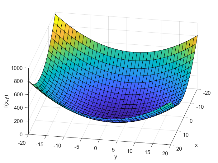
First, let us consider the following function

(1) $\begin{align*}f(x,y)=(x-2)^{2}+(y-2)^{2}\end{align*}$

where $x$ and $y$ are independent variables, and $f(x,y)\in \mathbb{R}$ is the function value. This function is shown in the figure below.

In the general case, the gradient of a function of two variables is a vector defined by

(2) $\begin{align*}g(x,y)=\nabla f(x,y)=\begin{bmatrix} \frac{\partial f}{\partial x} \\ \frac{\partial f}{\partial y} \end{bmatrix} \end{align*}$

where

$\nabla$ (nabla) is a mathematical symbol for the gradient.
$g(x,y)$ is the notation for the gradient vector.
$\frac{\partial f}{\partial x}$ and $\frac{\partial f}{\partial y}$ are the partial derivatives of $f$ with respect to $x$ and $y$ .

Next, let us compute the gradient of (1). The gradient is given by

(3) $\begin{align*}g(x,y)=\nabla f(x,y)=\begin{bmatrix} \frac{\partial f}{\partial x} \\ \frac{\partial f}{\partial y} \end{bmatrix} =\begin{bmatrix} 2(x-2) \\ 2(y-2) \end{bmatrix}\end{align*}$

Next, let us compute the gradient at the point $(x=10,y=10)$ . The gradient at this point is equal to

(4) $\begin{align*}g(10,10)=\nabla f(10,10)=\begin{bmatrix} 16 \\ 16 \end{bmatrix}\end{align*}$

This gradient vector is shown in the figure below (red arrow).

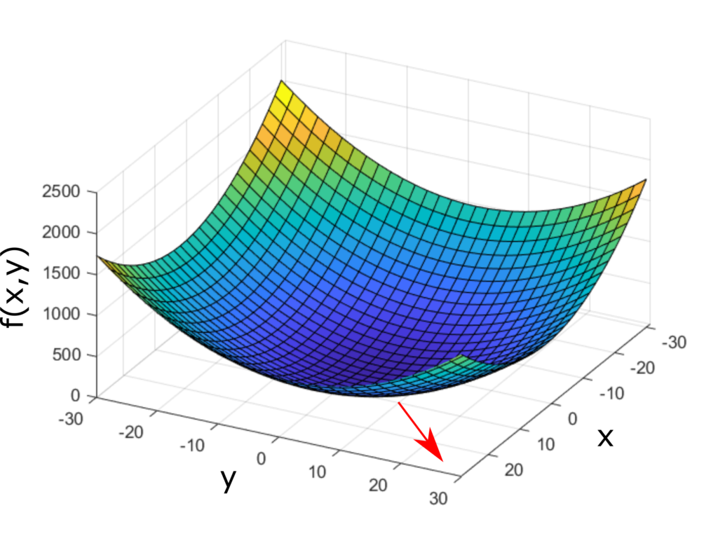
Figure 2: Illustration of the gradient vector of the function (1) at the point $x=10$ and $y=10$ . The gradient is illustrated by the red arrow.

Next, let us generalize the gradient definition. In the general case, the function $f$ depends on the $n$ variables: $x_{1}$ , $x_{2}$ , …, $x_{n}$ :

(5) $\begin{align*}f=f(x_{1},x_{2},x_{3},\ldots, x_{n})\end{align*}$

The gradient of the function $f$ is the $n$ -dimensional vector

(6) $\begin{align*}g(x_{1},x_{2},\ldots,x_{n})=\nabla f(x_{1},x_{2},\ldots,x_{n})=\begin{bmatrix} \frac{\partial f}{\partial x_{1}} \\ \frac{\partial f}{\partial x_{2}}\\ \vdots \\ \frac{\partial f}{\partial x_{n}} \end{bmatrix}\end{align*}$

Automatic Computation of Gradients in Python

To compute the gradients, we use Python’s symbolic computation library called SymPy. First, let us explain how to compute the gradients of the function

(7) $\begin{align*}f(x_{1},x_{2})=(x_{1}-2)^{2}+(x_{2}-2)^{2}\end{align*}$

The gradients are given by

(8) $\begin{align*}\nabla f(x_{1},x_{2}) =\begin{bmatrix} 2(x_{1}-2) \\ 2(x_{2}-2) \end{bmatrix} =\begin{bmatrix} 2x_{1}-4 \\ 2x_{2}-4 \end{bmatrix}\end{align*}$

The gradients in Python are computed as follows

# -*- coding: utf-8 -*-
"""
Computation of Symbolic Gradients in Python and 
Automatic Generation of Python Functions for Gradients

"""
import numpy as np
from sympy import *
init_printing()

# symbolic state vector
x = MatrixSymbol('x',2,1)

# nonlinear function 
f=Matrix([(x[0]-2)**2+(x[1]-2)**2])

# compute the gradient
g=f.jacobian(x)  

# compute the transpose
g=g.transpose()

First, we import the necessary functions and libraries. Then, we define the symbolic vector “x”. The entries of this vector are symbolic versions of $x_{1}$ and $x_{2}$ . Then, we define the nonlinear function “f”. To compute the gradient, we use the function “jacobian()”. The input of this function is the symbolic variable (vector) for computing the Jacobian matrix. The Jacobian of a scalar function is the gradient vector. The function “jacobian()” returns a row vector. That is why we need to transpose the result to obtain the gradient vector.

Next, we create a Python function that will return the numerical value of the gradient for the given numerical value of the symbolic vector “x”. The following Python script is used to achieve this task

gradientFunction=lambdify(x,g)
xValue=np.array([[10],[10]])
gradientNumericalValue=gradientFunction(xValue)

The function “lambidfy()” is used to convert symbolic expressions into Python functions. The first input argument is the symbolic variable (vector) and the second input argument is the symbolic expression. The “lambdify” function returns the Python function that can be used for computing the numerical value of the symbolic expression. We call this function by passing the numerical value of the symbolic vector.

Next, let us consider the second test case. Consider the following function

(9) $\begin{align*}f(x_{1},x_{2},x_{3},x_{4})=x_{1}x_{2}+\sin(x_{3})+x_{2}e^{x_{4}}\end{align*}$

The gradient is given by

(10) $\begin{align*}\nabla f =\begin{bmatrix} x_{2} \\ x_{1}+e^{x_{4}} \\ \cos(x_{3}) \\ x_{2}e^{x_{4}} \end{bmatrix}\end{align*}$

The following Python script is used to compute the gradient of the function (9).

# -*- coding: utf-8 -*-
"""
Computation of Symbolic Gradients in Python and 
Automatic Generation of Python Functions for Gradients

"""
import numpy as np
from sympy import *
init_printing()

# symbolic state vector
x = MatrixSymbol('x',4,1)

# nonlinear function 
f=Matrix([x[0]*x[1]+sin(x[2])+x[1]*E**(x[3])])

# compute the gradient
g=f.jacobian(x)  

# compute the transpose
g=g.transpose()


gradientFunction=lambdify(x,g)
xValue=np.array([[1],[1],[2],[3]])
gradientNumericalValue=gradientFunction(xValue)

Brief Summary of Gradients of Functions

Automatic Computation of Gradients in Python

admin

You might also like

Draw and Animate the Movement of Circles in Python and Pygame

Compute Fourier Series in Python by Using Symbolic Library and Generate Plots of Approximation Functions

Use Python and SymPy Function Lambdify() to Transform Symbolic Expressions and Symbolic Matrices to Python (Lambda) Functions