Compute Fourier Series in Python by Using Symbolic Library and Generate Plots of Approximation Functions – Fusion of Engineering, Control, Coding, Machine Learning, and Science

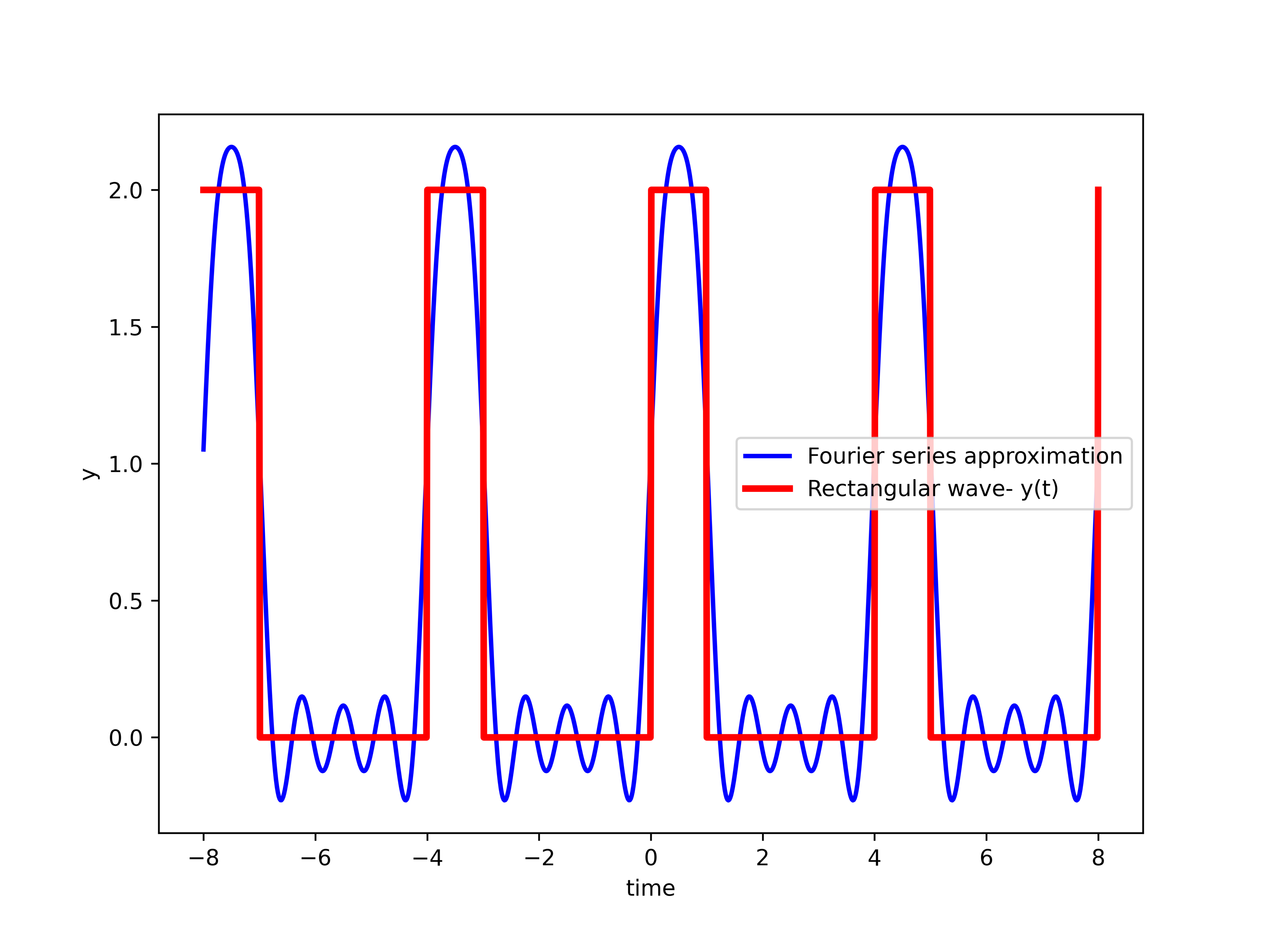
In this Python and signal processing tutorial, we explain how to symbolically compute the Fourier series expansion in Python and how to generate graphs of the Fourier series and related approximation functions. Although there are other methods for computing the Fourier series, such as for example a method based on numerical approximation of integrals for computing Fourier series expansion coefficients, in this tutorial, we use the method based on symbolic computation of Fourier series coefficients. Since this method is based on symbolic integration, it can help engineers, students, and professors obtain important insights into the analytic forms and formulas for Fourier series coefficients and functions. To perform symbolic computations, we use Python’s SymPy. By reading this tutorial, you will be able to generate the graph given below.

This graph shows the Fourier series approximation of the rectangular wave. Furthermore, you will be able to derive analytic functions involving complex exponentials and harmonics that are used to compute the Fourier series approximation shown in this graph.

Before reading this tutorial, we suggest to students that they thoroughly study our previous tutorial which concisely and clearly summarizes the Fourier series. The tutorial is given here. The YouTube tutorial accompanying this video tutorial is given below

Summary of Fourier Series

Let $y(t)$ be a periodic function. Then, the Fourier series of a periodic function $y(t)$ is defined by the following equation

(1) $\begin{align*}y(t)=\sum_{k=-\infty}^{+\infty} c_{k}e^{jk\omega_{0}t}\end{align*}$

where $j$ is the imaginary unit, $\omega_{0}=2\pi / T_{0}$ is the fundamental frequency, and $T_{0}$ is the fundamental period of the function $y(t)$ . The Fourier series coefficients $c_{k}$ are given by the following function

(2) $\begin{align*}c_{k}=\frac{1}{T_{0}}\int_{T_{0}}y(t)e^{-jk\omega_{0}t} \mathrm{d}t\end{align*}$

Python Script for Computing Fourier Series

The idea for computing the Fourier series is to symbolically integrate the Fourier series coefficients (2), and then to create a symbolic Fourier series expansion (1). We use the SymPy Python library for symbolic computation and integration. As a test case, we use the periodic rectangular wave function shown in the figure below.

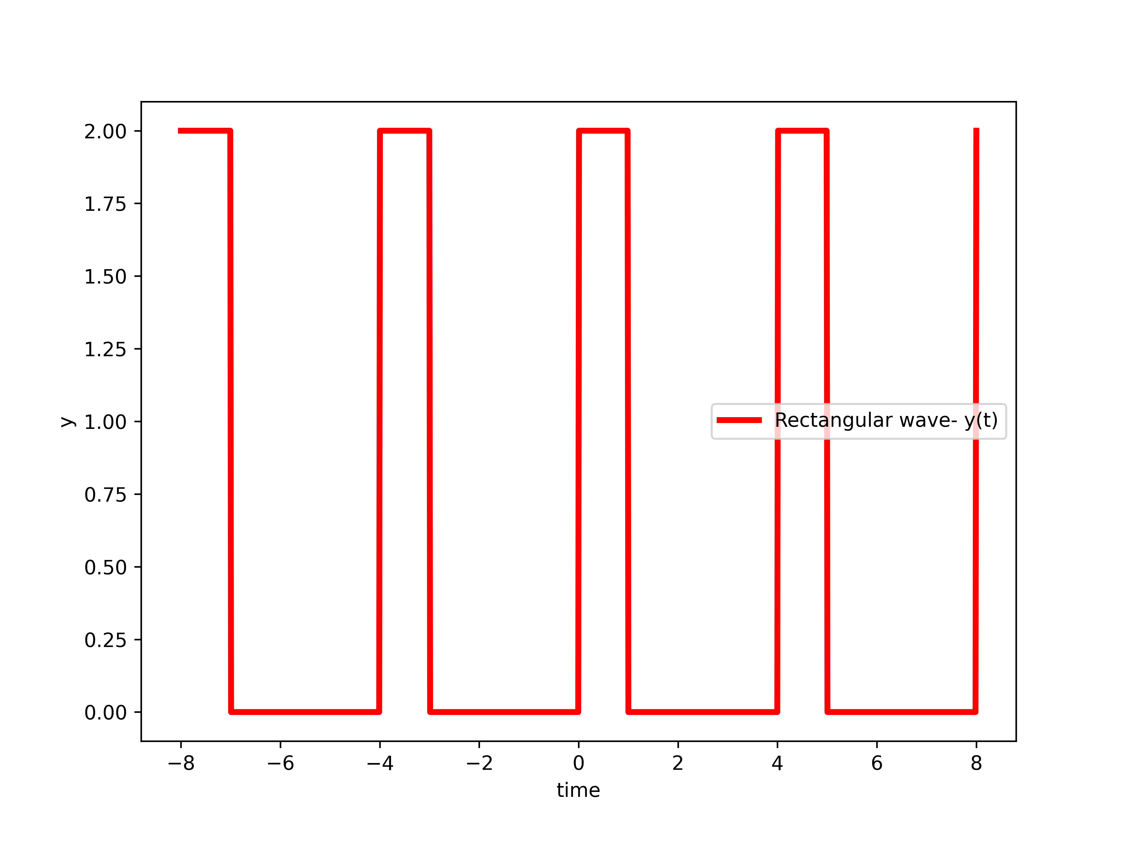
The fundamental period of this function is $T_{0}=4$ . First, we need to import the necessary library and define the main parameters and variables. The Python script is given below.

# Fourier Series in Python 
# Here, we compute the Fourier series of the periodic 
# rectangular wave
import numpy as np
from sympy import *
import matplotlib.pyplot as plt
# time symbol
t = Symbol('t', real=True)
# fundamental period
To=4
# fundamental frequency
omega0=2*pi/To
# amplitude of the wave
a=2

We import the NumPy and SymPy libraries, as well as the plotting function pyplot() from matplotlib. Next, we define the symbolic variable $t$ for time. Then, we define the fundamental period, fundamental frequency, and amplitude of the wave.

Next, we need to compute the Fourier series coefficients by symbolically computing the integral given by (2). Over here, for clarity, we repeat the integral

(3) $\begin{align*}c_{k}=\frac{1}{T_{0}}\int_{T_{0}}y(t)e^{-jk\omega_{0}t} \mathrm{d}t\end{align*}$

By looking at the shape of the function in Fig. 1, the integral takes the following form

(4) $\begin{align*}c_{k} & =\frac{1}{T_{0}}\int_{0}^{T_{0}}y(t)e^{-jk\omega_{0}t} \mathrm{d}t \\& = \frac{1}{T_{0}}\int_{0}^{4}y(t)e^{-jk\omega_{0}t} \mathrm{d}t \\& = \frac{1}{4}\int_{0}^{1}2\cdot e^{-jk\omega_{0}t} \mathrm{d}t + \frac{1}{4}\int_{1}^{4} 0 \cdot e^{-jk\omega_{0}t} \mathrm{d}t \\& = \frac{1}{4}\int_{0}^{1}2\cdot e^{-jk\omega_{0}t} \mathrm{d}t\end{align*}$

Or in the parameterized form

(5) $\begin{align*}c_{k} & = \frac{1}{T_{0}}\int_{0}^{1}a\cdot e^{-jk\omega_{0}t} \mathrm{d}t\end{align*}$

where $a=2$ is the amplitude and $T_{0}=4$ is the fundamental period. The Python script given below is used to compute (5).


# Number of Fourier series coefficients 
# -k until +k, that is, in total 2*k+1 coefficient
k=4
# create the vector for storing the coefficients
coffNumber=np.arange(-k,k+1,1)
computedCoefficients=[]

# compute the coefficients by using the definition
for index in coffNumber:
    # use the definition
    coeffComputed=((1/To)*integrate(a*exp((-index*I*omega0*t)),(t, 0, 1))).simplify().evalf(6)
    computedCoefficients.append(coeffComputed)

In this script, we compute $2\cdot k+1$ coefficients. In the for loop, to compute the coefficients, we use the SymPy function “integrate”. The first argument of this function is the mathematical function that needs to be integrated. We specify the integral given by (5). The variable “index” is the coefficient number $k$ . The constant “I” is the SymPy constant for the imaginary unit $j$ . The second argument is the tuple. The first element of this tuple is the variable used for integration. The second and third elements are integration bounds. After we integrate the function, we divide the result by $1/T_{0}$ , and we simplify and evaluate the expression, such that we can have a more compact expression. Finally, we append the list for storing the computed coefficients.

After we computed the coefficients, we compute the Fourier series expansion (finite number of terms)

(6) $\begin{align*}y(t)=\sum_{k=-n}^{+n} c_{k}e^{jk\omega_{0}t}\end{align*}$

In our implementation, the number $n$ is actually denoted by $k$ . The following Python script is used to compute the approximation (6):

# create a symbolic function that approximates the series
approximateFunction=0
data=zip(coffNumber,computedCoefficients)
for coeffNumber,coeffValue in data:
    approximateFunction=approximateFunction+coeffValue*E**(I*coeffNumber*omega0*t)

The computed function is

(7) $\begin{align*}y_{4}(t) & =\left(-0.106103 - 0.106103 i\right) e^{\frac{3 i \pi t}{2}} + \left(0.31831 - 0.31831 i\right) e^{\frac{i \pi t}{2}} \\ & - 0.31831 i e^{i \pi t} + 0.5 + 0.31831 i e^{- i \pi t} \\& + \left(0.31831 + 0.31831 i\right) e^{- \frac{i \pi t}{2}} + \left(-0.106103 + 0.106103 i\right) e^{- \frac{3 i \pi t}{2}}\end{align*}$

Here, it should be kept in mind that the Fourier coefficients for $k=\pm 4$ are equal to zero, consequently, the corresponding terms are equal to zero.

Next, we need to graphically represent the approximation results. This is done by using the Python script given below.


# create a function that will return the 
# value of the approximation for the given time instant
approximationFun=lambdify(t,approximateFunction)
timeVector=np.linspace(-2*To,2*To,1000)
functionValues=approximationFun(timeVector)
# need to extract a real value since there is a very 
# small complex value
functionValues=functionValues.real

# create a periodic rectangular wave function
functionValuesTrue=np.zeros(shape=timeVector.shape)
for i in range(len(timeVector)):
    if((timeVector[i]%4)<=1):
        functionValuesTrue[i]=a
    
        
# plot the results 
plt.figure(figsize=(8,6))
plt.plot(timeVector,functionValues,'b',linewidth=2,label='Fourier series approximation')
plt.plot(timeVector,functionValuesTrue,'r',linewidth=3,label='Rectangular wave- y(t)')
plt.xlabel('time')
plt.ylabel('y')
plt.legend()
plt.savefig('rectWave.png',dpi=600)
plt.show()

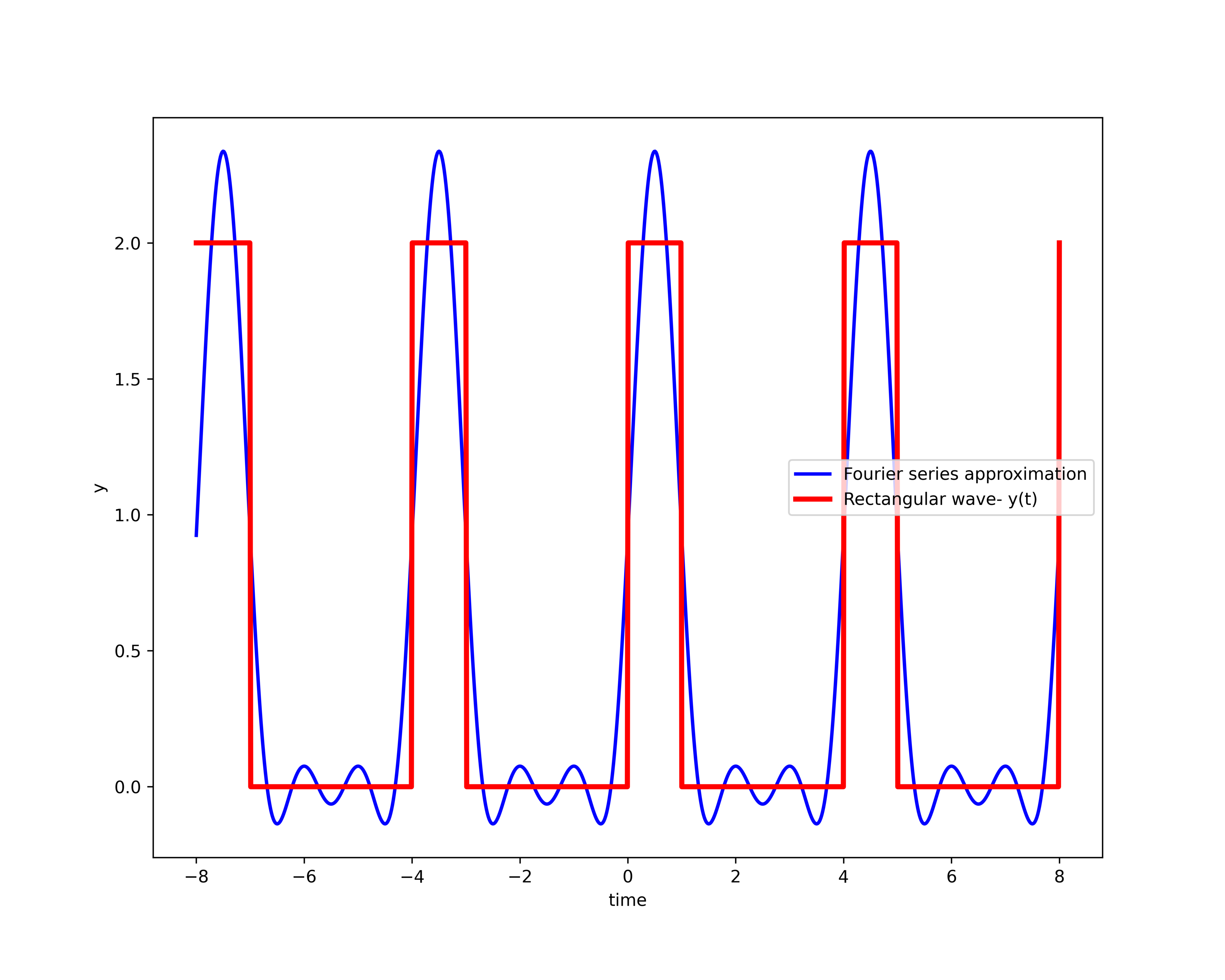
We create a Python function out of the computed symbolic Fourier series function “approximateFunction”. To do that, we use the function “lambdify()”. This function creates the function “approximationFun” that accepts as an argument time $t$ , and that returns the value of the approximation given by (7) for given time $t$ . This function is used to generate the vector of function values for plotting. We also create a rectangular wave and the corresponding vector of values for plotting. Finally, we plot the result. The generated figure is shown below.

Summary of Fourier Series

Python Script for Computing Fourier Series

admin

You might also like

Automatic State-Space Derivation and Simulation of Nonlinear Dynamical Systems in Python with Inverted Pendulum on a Cart Example

Pole Placement With Integral Control Action to Eliminate Steady-State Error (State-Space Control Design)

Simulation of Transfer Function Response in Python – Control Engineering Tutorials