Simulation of Transfer Function Response in Python – Control Engineering Tutorials

In this control engineering and control theory tutorial, we will learn

1. How to define a transfer function of a control system in Python by using the Python Control Systems Library
2. How to simulate the step response of a transfer function in Python by using the Python Control Systems Library
3. How to simulate the initial state response of a transfer function in Python by using the Python Control Systems Library
4. How to simulate the response of a transfer function to arbitrary control inputs in Python by using the Python Control Systems Library

This tutorial is based on the Python Control Systems Library whose page is given here. The YouTube tutorial accompanying this page is given below.

Library Installation and Definition of Transfer Functions

To install this library, open the command prompt or the Anaconda command line environment and type

pip install control

For advanced functionality, you can also try to run

pip install slycot   # optional

However, the installation of “slycot” is not necessary for this tutorial.

The following Python script will import the necessary libraries and will define a plotting function that is used in this tutorial.

import matplotlib.pyplot as plt
import control as ct
import numpy as np

# this function is used for plotting of responses 
# it generates a plot and saves the plot in a file 

# xAxisVector - time vector
# yAxisVector - response vector
# titleString - title of the plot
# stringXaxis - x axis label 
# stringYaxis - y axis label
# stringFileName - file name for saving the plot, usually png or pdf files

def plottingFunction(xAxisVector,yAxisVector,titleString,stringXaxis,stringYaxis,stringFileName):
    plt.figure(figsize=(8,6))
    plt.plot(xAxisVector,yAxisVector, color='blue',linewidth=4)
    plt.title(titleString, fontsize=14)
    plt.xlabel(stringXaxis, fontsize=14)
    plt.ylabel(stringYaxis,fontsize=14)
    plt.tick_params(axis='both',which='major',labelsize=14)
    plt.grid(visible=True)
    plt.savefig(stringFileName,dpi=600)
    plt.show()

First, we import the Matplotlib plotting function. After that we import the Control Systems Library as “ct” (this is the standard convention for importing this library). Finally, we import the NumPy library. After that, we define a function that is used for plotting of time sequences of inputs, outputs, and states. This function will store the results in the specified “png” file such that you can include the file in your report or a scientific article.

Let us consider the following transfer function

(1)  

where , , and , , are the coefficients of the transfer function. To define such a transfer function, we use the following function

W=ct.tf(num,den)

where “num” and “den” are two Python lists defining the coefficients in the numerator and denominator of the transfer function. The first entries of the two lists are the coefficients with the largest indices, and the entries are ordered in descending order. For example, in the case of the transfer function (1), the lists will be

(2)  

For example, consider the following transfer function

(3)  

Then the Python code defining this function is

# define a transfer function
num=[2,4]
den=[1,2,4]

# here we define the transfer function
W=ct.tf(num,den)
print(W)

Step Response of Transfer Functions in Python

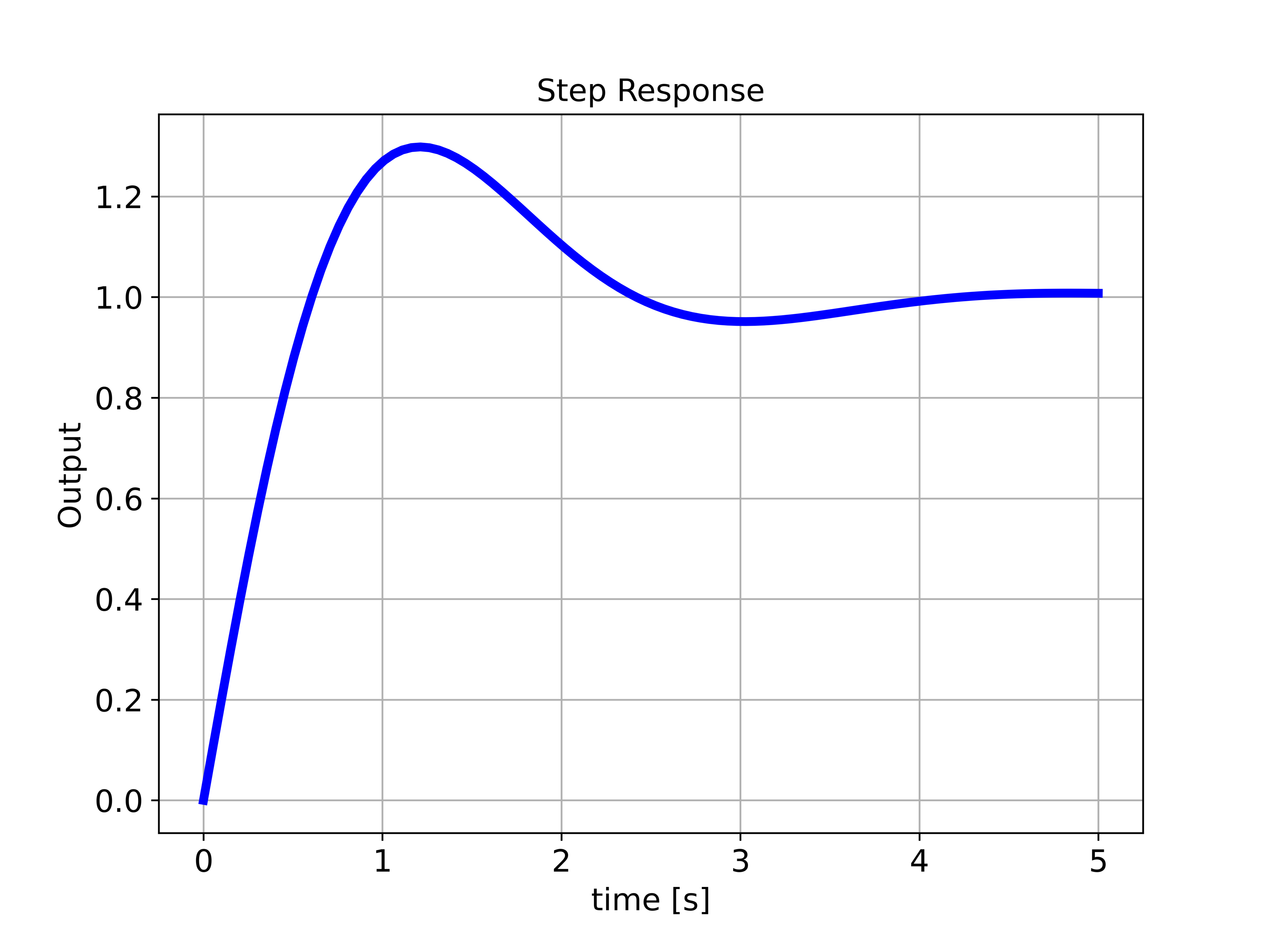
Here, we explain how to compute the step response of the transfer function (3). The code is given below.

# define a transfer function
num=[2,4]
den=[1,2,4]

# here we define the transfer function
W=ct.tf(num,den)
print(W)

###############################################################################
# simulate the step response
###############################################################################
timeVector=np.linspace(0,5,100)
timeReturned, systemOutput = ct.step_response(W,timeVector)

# plot the step response
plottingFunction(timeReturned,systemOutput,
                 titleString='Step Response',
                 stringXaxis='time [s]' , 
                 stringYaxis='Output',
                 stringFileName='stepResponse.png',)
###############################################################################

To simulate the step response we use the function “ct.step_response(W,timeVector)”. The first input argument of this function is the transfer function and the second input argument is the time vector (NumPy array) for simulation. The output is the time array used during the simulation and the computed step response. The figure shown below is the simulated step response.

Response of Transfer Functions to Arbitrary Control Inputs and Initial States in Python

Here, we explain how to simulate the response of the transfer function to arbitrary control inputs and initial states. The Python script is given below.

###############################################################################
# Simulate the system response to a specific input
###############################################################################
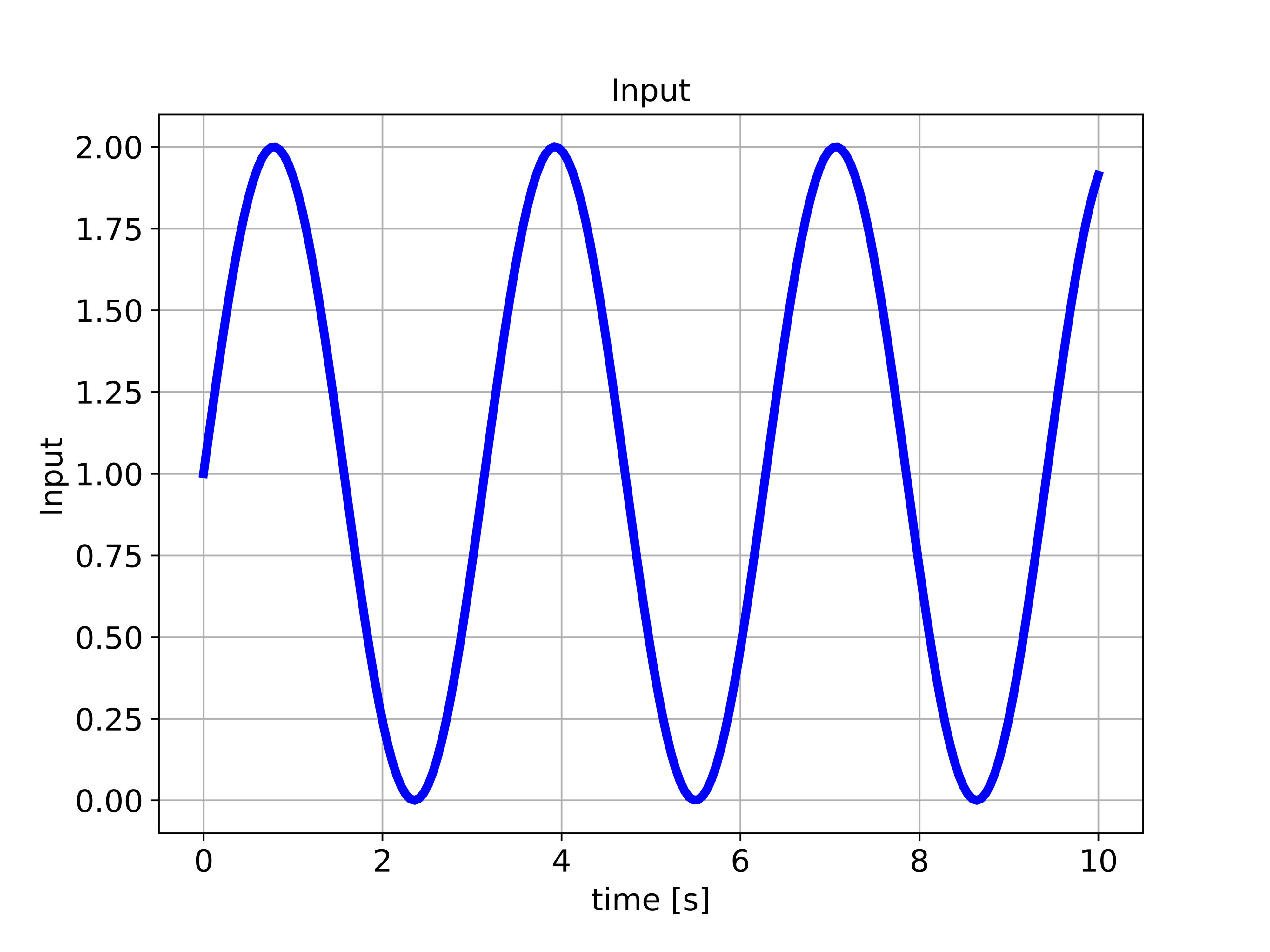
# generate the input vector
timeVector2=np.linspace(0,10,200)
inputVector2=np.sin(2*timeVector2)+np.ones(timeVector2.shape)

# initial state
x0=np.array([[-0.2],[0]])

# plot the input vector
plottingFunction(timeVector2,inputVector2,
                 titleString='Input',
                 stringXaxis='time [s]' , 
                 stringYaxis='Input', 
                 stringFileName='appliedInputNew.png')

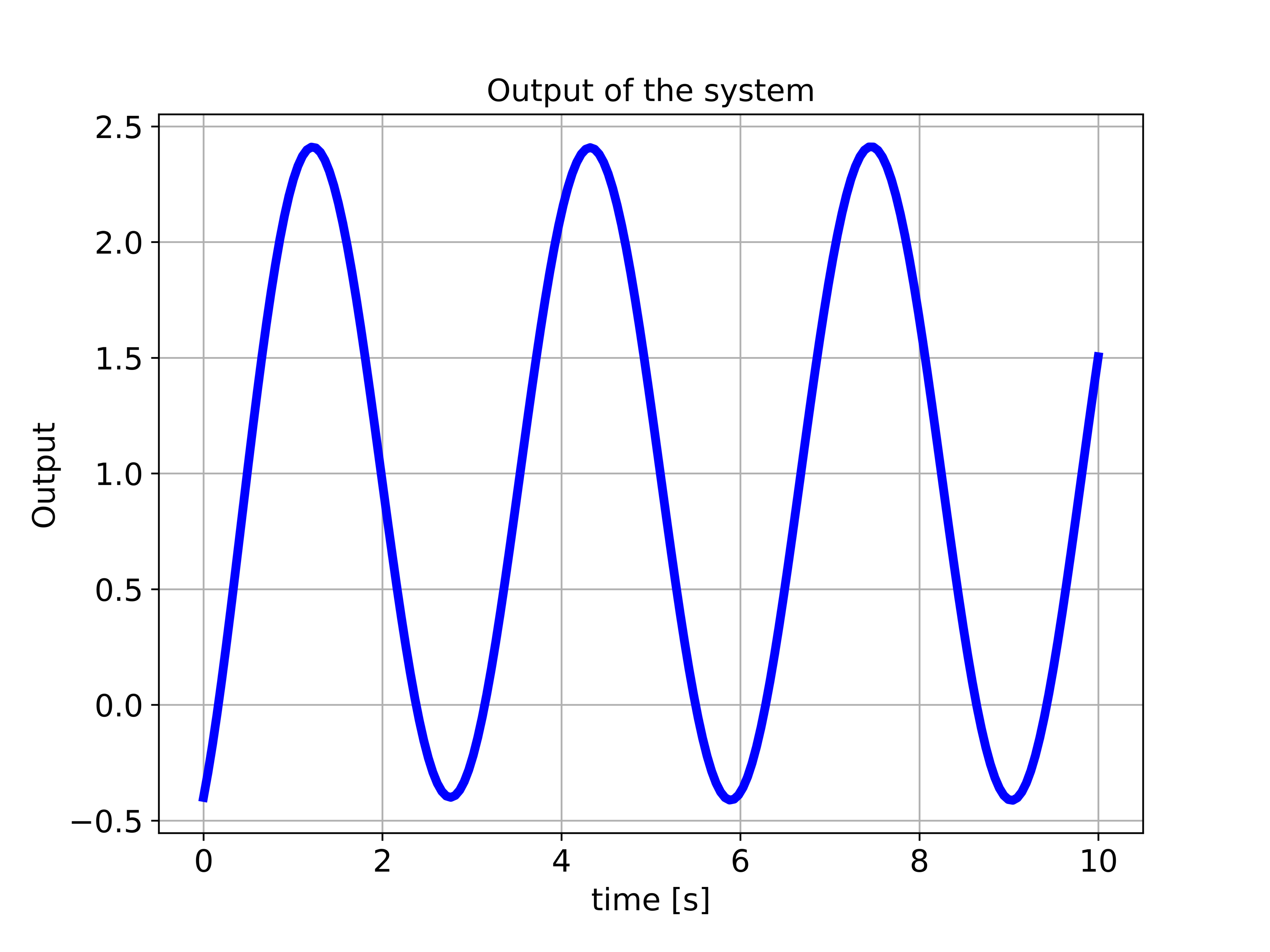
# compute the response of the system to the specific input
timeReturned2, systemOutput2 = ct.forced_response(W,timeVector2,inputVector2,x0)
plottingFunction(timeReturned2,systemOutput2,
                 titleString='Output of the system',
                 stringXaxis='time [s]' , 
                 stringYaxis='Output', 
                 stringFileName='outputSinusoidalNew.png')
###############################################################################

First, we define the time array and the control input array. Then, we define the initial state. We use the function “ct.forced_response()” to compute the output response. The first input argument of this function is the transfer function . The second input argument is the time array used for simulation. The third input argument is the applied control input array. The final input argument is the initial state. The function “ct.forced_response()” returns the time array used for simulation and the simulated output of the system. The applied control input is shown in the figure below.

The simulated output is given in the figure below.

Response of the Transfer Function to Arbitrary Initial State in Python

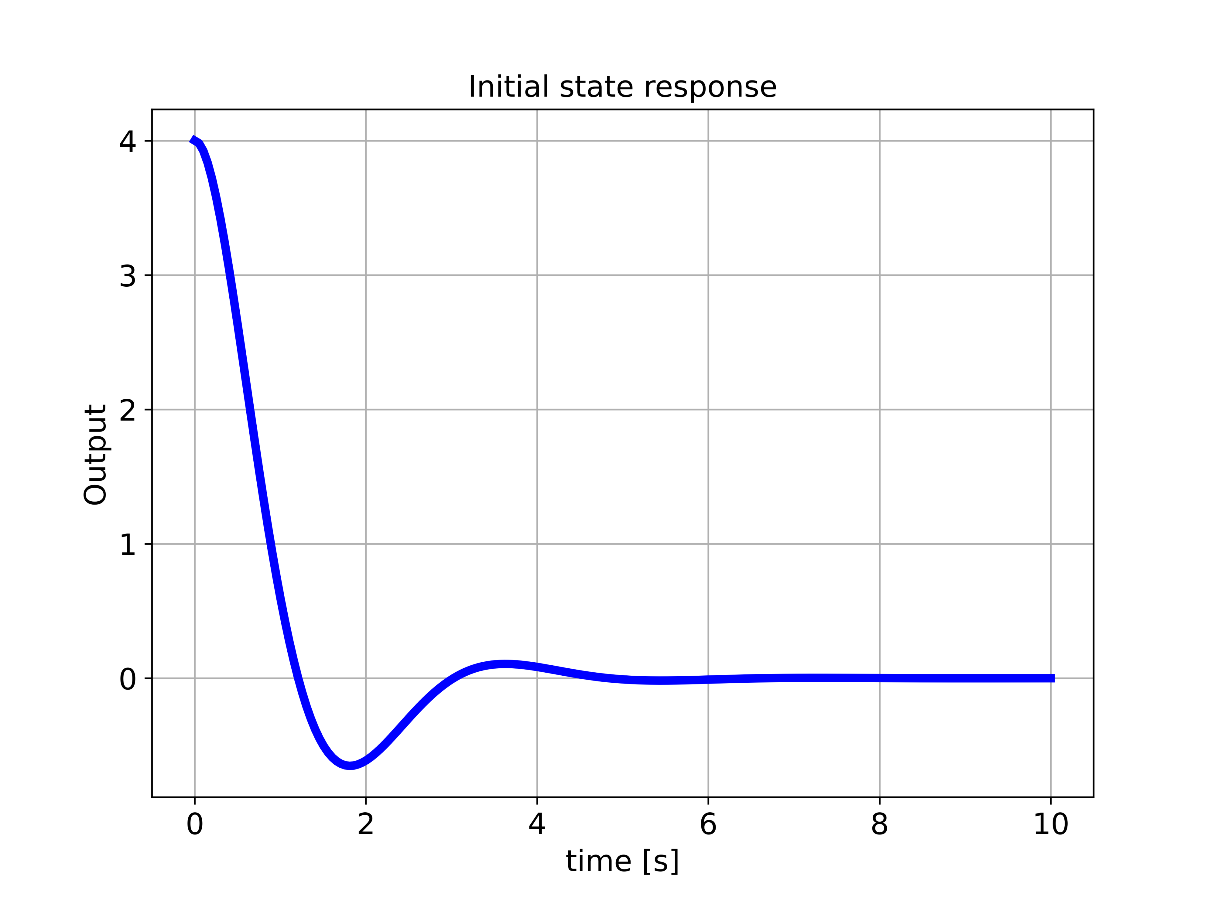
Here, we explain how to simulate the response of the transfer function to an arbitrary initial state. The Python script is given below.

###############################################################################
# Initial state response
###############################################################################
timeVector3=np.linspace(0,10,200)
initialState=np.array([[2],[0]])

timeReturned3, systemOutput3 = ct.initial_response(W,timeVector3,initialState)
plottingFunction(timeReturned3,systemOutput3,
                 titleString='Initial state response',
                 stringXaxis='time [s]' , 
                 stringYaxis='Output', 
                 stringFileName='outputInitialNew.png')

We first, define the time array and the initial state. We use the function “ct.initial_response()” to simulate the response of the transfer function to the defined initial state. The first input argument of the function “ct.initial_response()” is the transfer function. The second input argument is the time array. The third input argument is the defined initial state. The output of the system is shown in the figure below. Since the system is asymptotically stable, the output of the system converges to zero.