Definition and Simulation of State-Space Models of Linear Systems in Python by Using Control Systems Library

In this control engineering and control theory tutorial, we explain how to define and simulate state-space models of linear dynamical systems in Python. Furthermore, we explain how to perform basic operations on state-space models in Python. The approach presented in this webpage tutorial is based on the Python Control Systems Library. More precisely, in this webpage tutorial, we explain

1. How to define state-space models in Python.
2. How to convert state-space models to transfer function models and back in Python.
3. How to simulate the step response of state-space models in Python.
4. How to compute poles, zeros, natural frequencies, and damping ratios of state-space models in Python.
5. How to discretize continuous-time state-space models in Python.

The YouTube tutorial accompanying this webpage is given below.

Installation of the Control Systems Library and Definition of State-Space Models

To install the Control Systems Library, open a terminal and type

pip install control

After installing the library, open a new Python script, and type

import matplotlib.pyplot as plt
import control as ct
import numpy as np

# this function is used for plotting of responses 
# it generates a plot and saves the plot in a file 

# xAxisVector - time vector
# yAxisVector - response vector
# titleString - title of the plot
# stringXaxis - x axis label 
# stringYaxis - y axis label
# stringFileName - file name for saving the plot, usually png or pdf files

def plottingFunction(xAxisVector,yAxisVector,titleString,stringXaxis,stringYaxis,stringFileName):
    plt.figure(figsize=(8,6))
    plt.plot(xAxisVector,yAxisVector, color='blue',linewidth=4)
    plt.title(titleString, fontsize=14)
    plt.xlabel(stringXaxis, fontsize=14)
    plt.ylabel(stringYaxis,fontsize=14)
    plt.tick_params(axis='both',which='major',labelsize=14)
    plt.grid(visible=True)
    plt.savefig(stringFileName,dpi=600)
    plt.show()

First, we import the plotting function. Then by using “import control as ct”, we import the Control Systems Library. Here it should be emphasized that it is the standard convention to import the Control Systems Library as “ct”. Finally, import the NumPy library. After that, we define a function for generating plots of simulated responses of state-space models. This function generates a plot and saves it in a file specified by the user. We will use this function later on in this tutorial.

In this tutorial, we consider linear state-space models with the following form

(1)  

The Python script shown below defines a state-space model.

A=np.array([[0, 1],[-4, -2]])
B=np.array([[0],[1]])
C=np.array([[1,0]])
D=np.array([[0]])

sysStateSpace=ct.ss(A,B,C,D)

print(sysStateSpace)

First, we define the system state-space matrices , , , and . To define the state-space model we use the function “ct.ss()”. The input arguments of this function are the system matrices.

Step Response of State-Space Model and Basis Operations

First, we explain how to compute the step response of the state-space model in Python. The Python script is given below.

timeVector=np.linspace(0,5,100)
timeReturned, systemOutput = ct.step_response(sysStateSpace,timeVector)

# plot the step response
plottingFunction(timeReturned,systemOutput,
                 titleString='Step Response',
                 stringXaxis='time [s]' , 
                 stringYaxis='Output',
                 stringFileName='stepResponseSS.png')

# obtain the basic information about the step response
stepInfoData = ct.step_info(sysStateSpace)

First, we define a time vector (array) for simulation. Then, to compute the step response, we use the function “ct.step_response()”. The first input argument of this function is the state-space model, and the second input is the time array for simulation. The function “ct.step_response()” returns two arrays. The first array is the time vector used for simulation and the second array is the computed step response. We generate a plot of the computed step response by calling the function “plottingFunction” which is defined in the previous section. The resulting graph is shown in the figure below.

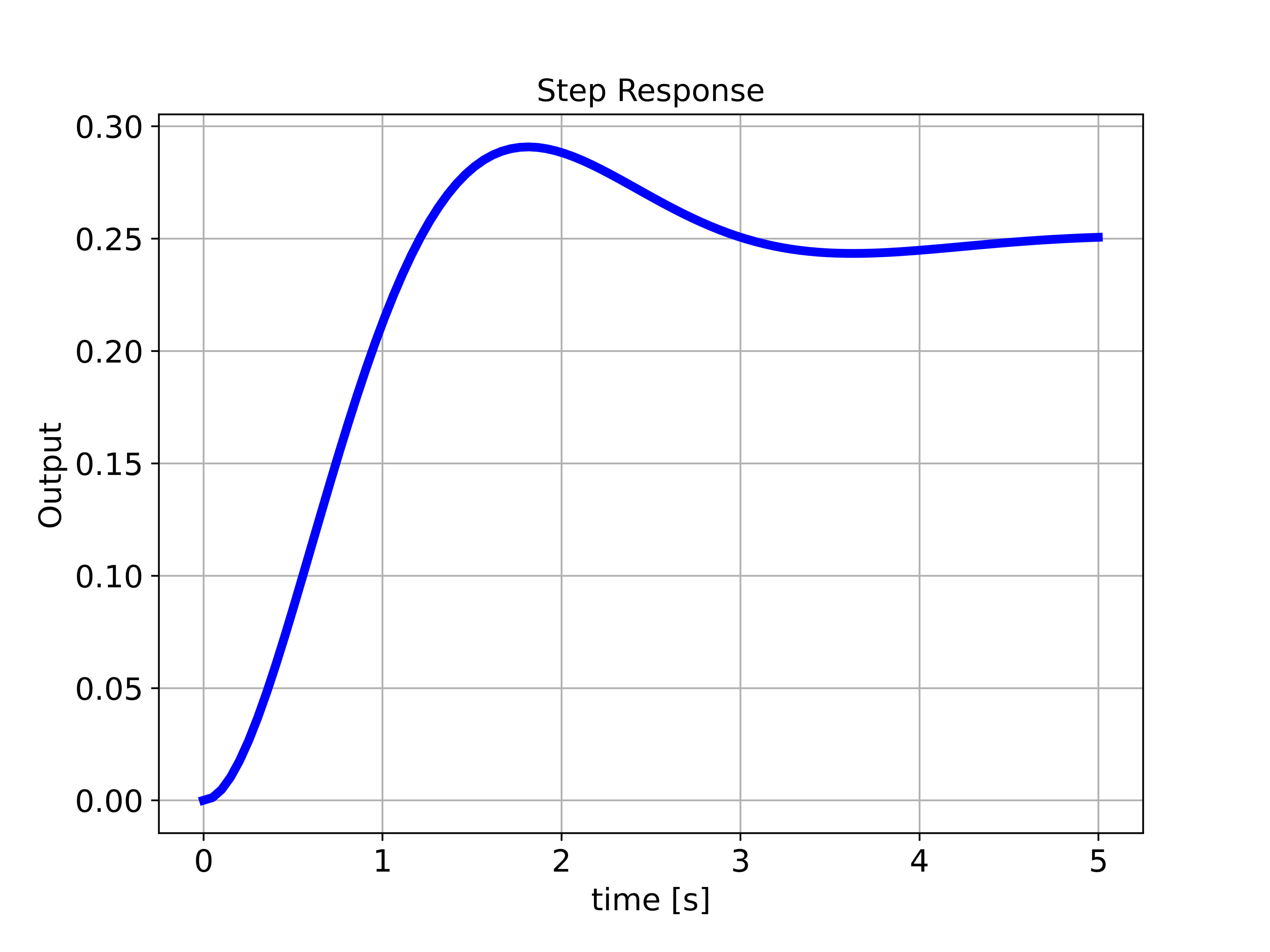
The function “ct.step_info()” is very useful for investigating the properties of the simulated step response, such as rise time, settling time, overshoot, undershoot, peak, peak time, and steady-state value. This function returns the following output

{'RiseTime': 0.837303670179653,
 'SettlingTime': 4.046967739201657,
 'SettlingMin': 0.23487229056187914,
 'SettlingMax': 0.2907583732260488,
 'Overshoot': 16.303349290419522,
 'Undershoot': 0,
 'Peak': 0.2907583732260488,
 'PeakTime': 1.814157952055915,
 'SteadyStateValue': 0.25}

We can convert state-space models to transfer functions and vice versa, by using the following Python script

# convert state-space to transfer function
transferFunction1=ct.ss2tf(sysStateSpace)
print(transferFunction1)

# convert transfer function to state-space 
sysStateSpace2=ct.tf2ss(transferFunction1)
print(sysStateSpace2)

The Python script given below will compute the natural frequency, damping ratio, poles, and zeros of the state-space model

# Compute natural frequencies, damping ratios, and poles of a system
ct.damp(sysStateSpace, doprint=True)

# Compute poles
ct.poles(sysStateSpace)

# Compute zeros
ct.zeros(sysStateSpace)

# Pole-zero map 
ct.pzmap(sysStateSpace)

# sisotool - similar to the MATLAB's sisotool collection of plots 

ct.sisotool(sysStateSpace)

The function “ct.sisotool()” generates the Bode and Root locus plots of the state-space model.

We can also discretize the continuous-time state-space model. The Python script given below discretizes the state-space models and simulates the step response of the discretized state-space model.

# discretization time
sampleTime=0.1
# discretize the system dynamics
# method='zoh' - zero order hold discretization
# method='bilinear' - bilinear discretization
sysStateSpaceDiscrete=ct.sample_system(sysStateSpace,sampleTime,method='zoh') 

# check if the system is in discrete-time
sysStateSpaceDiscrete.isdtime()

print(sysStateSpaceDiscrete)

# compute the step response

timeVector2=np.linspace(0,5,np.int32(np.floor(5/sampleTime)+1))
timeReturned2, systemOutput2 = ct.step_response(sysStateSpaceDiscrete,timeVector2)

# plot the step response
plottingFunction(timeReturned2,systemOutput2,titleString='Step Response',stringXaxis='time [s]' , stringYaxis='Output',stringFileName='stepResponse.png')

The function “ct.sample_system” is used to discretize the state-space model. The first input of this function is the continuous-time state-space model and the second input is the discretization method. We can select between the zero-order hold (denoted by “zoh”) and bilinear discretization methods.