 by
by
In this physics, dynamical systems, and control engineering tutorial, you will learn
- How to automatically derive state-space models of nonlinear systems starting from the equations of motion. You will learn how to completely automatize the derivation process by using Python and Python’s symbolic computation library called SymPy.
- How to simulate the derived nonlinear state-space model in Python. You will also learn how to simulate the state-space model for arbitrary control inputs.
As a test case, we use a nonlinear inverted pendulum on a cart system. For brevity, in this tutorial, we call this system the cart-pendulum system. This system is a very important example of a non-trivial nonlinear system that is often used as a benchmark of different control and estimation algorithms.
The state-space model of the cart-pendulum system has four state variables. For this system, the derivation of the nonlinear state-space model from the equations of motion is not trivial and if a person is doing the derivations by hand, most likely he or she will make an error. Motivated by this, we created this tutorial that explains how to completely automatize the derivation process and how to easily simulate the nonlinear dynamics of this system in Python. Everything explained in this video tutorial can be generalized to more complex dynamical systems, such as UAVs, mobile robots, robotic arms, etc.
In the second part of this tutorial, given here, we explain how to animate the motion of the cart-pendulum system in Python by using the library called Pygame.
The GitHub page accompanying this webpage tutorial is given here. The YouTube video accompanying the first tutorial part is given below.
The YouTube tutorial accompanying the second tutorial part is given below.
Cart-Pendulum Equations of Motion
The cart pendulum system is given in the figure below.
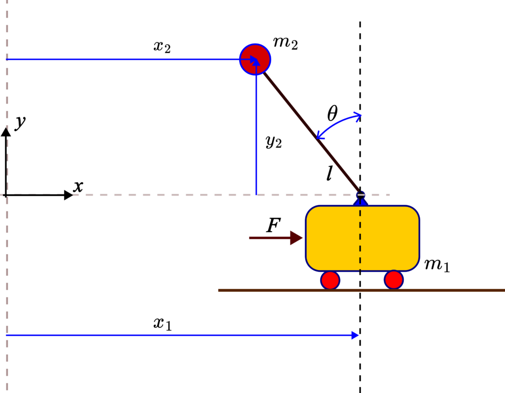
The system is made of a cart with the mass of  . The control force
  is applied to the cart. A ball of mass
  is rigidly attached to the rod of length
  . The pendulum is a rigid connection composed of the rod and the ball. The pendulum rotates around its base which is placed on the cart. During the modeling process of this system, we neglect the mass of the rod. The variable
  is the
  -axis position of the cart. The variable
  is the -axis position of the ball. The variable
  denotes the
  -position of the ball. The variable
  denotes the angle of the pendulum with respect to the vertical direction. The positive angle is in the counter-clock direction.
In our previous tutorial, given here, we derived the equations of motion of this system. The equations have the following form
(1) 
where  is the gravitational acceleration constant,
  is the first derivative of with respect to time
  ,
,  is the second derivative of with respect ,
  is the first derivative of , and
  is the second derivative of with respect to .
Derivation of State-Space Model of Cart-Pendulum System
Our goal is to derive the state-space model of the cart-pendulum system. First, let us introduce the state-space variables:
(2) 
By using the state-space variables (2), the equations of motion become
(3) 
To derive the state-space model, we need to solve these two equations for  and
and  . We can do this by hand. However, it will take a significant amount of time to perform this task. In addition, we will most likely make an error. Instead of doing this by hand, in the sequel we will learn how to automatically solve these two equations in Python and how to implement the state-space model.
Before continuing with this tutorial, we strongly suggest to the interested reader to thoroughly go over our previous tutorials on symbolic computations in Python by using SymPy. These tutorials will help the interested reader to better understand the material presented in the sequel. The tutorials are given below:
- Solve Systems of Equations Analytically in Python by Using Symbolic Library
- Use Python and SymPy Function Lambdify() to Transform Symbolic Expressions and Symbolic Matrices to Python (Lambda) Functions
The following Python script will define the symbolic variables, and solve the system of nonlinear equations 1 for and .
# import the necessary libraries
# we need numpy since we need to substitute symbolic variables by
# real numbers
import numpy as np
# we need odeint() to integrate the state-space model
from scipy.integrate import odeint
# we need the ploting function
import matplotlib.pyplot as plt
# we import the complete SymPy library to simplify the notation
from sympy import *
# we call this function to enable nice printing of symbolic expressions
init_printing()

###############################################################################
# START: this part of the code file is used to symbolically solve the equations
# of motion in order to define the state-space model
###############################################################################

# create the symbolic parameter variables
m1,m2,l,g=symbols('m1 m2 l g')
# symbolic force
F=symbols('F')
# state variables
z1,z2,z3,z4=symbols('z1 z2 z3 z4')

# derivatives
dz2, dz4 =symbols('dz2 dz4')

# first equation
e1=(m1+m2)*dz2-m2*l*dz4*cos(z3)+m2*l*(z4**2)*sin(z3)-F
# second equation
e2=l*dz4-dz2*cos(z3)-g*sin(z3)

# define and solve the equations
result=solve([e1, e2], dz2,dz4 , dict=True)

# first equation
dz2Solved=simplify(result[0][dz2])

# second equation
dz4Solved=simplify(result[0][dz4])
First, we import the necessary libraries. We import NumPy and SymPy libraries. From “scipy.integrate” we import the function “odeint()”. This function is used to integrate the derived nonlinear state-space model. We also import the plotting function. We call the function “init_printing()” that is used for generating nice prints of symbolic expressions.
We then define the symbolic variables: system parameters , , , and , control force , and state-space variables  and
and  . Finally, we define the symbolic variables that denote the derivatives of
  and . Finally, we define the symbolic equations that represent the equations (3). We use the function “solve” to compute the derivates of and and simplify the expressions. The computed expressions are
(4) 
The complete state vector is
(5) 
The state-space model is
(6) 
Next, we use the derived symbolic expressions to simulate the state-space model
# define the numerical values of the parameters
lV=1
gV=9.81
m1V=10
m2V=1
# substituted them in the equations
dz2Solved=dz2Solved.subs(l,lV).subs(g,gV).subs(m1,m1V).subs(m2,m2V)
dz4Solved=dz4Solved.subs(l,lV).subs(g,gV).subs(m1,m1V).subs(m2,m2V)

# create the Python functions that return the numberical values
functionDz2=lambdify([z1,z2,z3,z4,F],dz2Solved)
functionDz4=lambdify([z1,z2,z3,z4,F],dz4Solved)

# this function defines the state-space model, that is, its right-hand side
# z is the state
# t is the current time - internal to solver
# timePoints - time points vector necessary for interpolation
# forceArray - time-varying input
def stateSpaceModel(z,t,timePoints,forceArray):
    # interpolate input force values
    # depending on the current time
    forceApplied=np.interp(t,timePoints, forceArray)
    # NOTE THAT IF YOU KNOW THE ANALYTICAL FORM OF THE INPUT FUNCTION
    # YOU CAN JUST WRITE THIS ANALYTICAL FORM AS A FUNCTION OF TIME
    # for example in our case, we can also write
    # forceApplied=np.sin(t)+np.cos(2*t)
    # and you do not need to specity forceArray as an input to the function
    # HOWEVER, IF YOU DO NOT KNOW THE ANALYTICAL FORM YOU HAVE TO USE OUR APPROACH
    # AND INTERPOLATE VALUES
    # right-side of the state equation
    dz2Value=functionDz2(z[0],z[1],z[2],z[3],forceApplied)
    dz4Value=functionDz4(z[0],z[1],z[2],z[3],forceApplied)
    dzdt=[z[1],dz2Value,z[3],dz4Value]
    return dzdt


# define the simulation parameters
startTime=0
endTime=25
timeSteps=5000

# simulation time array
# we will obtain the solution at the time points defined by
# the vector simulationTime
simulationTime=np.linspace(startTime,endTime,timeSteps)

# define the force input
#forceInput = np.sin(simulationTime)+np.cos(2*simulationTime)
forceInput = np.zeros(shape=(simulationTime.shape))

# plot the applied force
plt.plot(simulationTime, forceInput)
plt.xlabel('time')
plt.ylabel('Force - [N]')
plt.savefig('inputSequence.png',dpi=600)
plt.show()

# define the initial state for simulation
initialState=np.array([0,0,np.pi/3,0])

# generate the state-space trajectory by simulating the state-space model
solutionState=odeint(stateSpaceModel,initialState,
                     simulationTime,
                     args=(simulationTime,forceInput))

# save the simulation data
# the save file is opened by another Python script that is used
# to animate the trajectory
np.save('simulationData.npy', solutionState)

# plot the state trajectories
# cart state trajectories
plt.figure(figsize=(10,8))
plt.plot(simulationTime, solutionState[:,0],'b',linewidth=4,label='z1')
plt.plot(simulationTime, solutionState[:,1],'r',linewidth=4,label='z2')
plt.xlabel('time',fontsize=16)
plt.ylabel('Cart states',fontsize=16)
plt.legend(fontsize=14)
plt.tick_params(axis='both', which='major', labelsize=14)
plt.grid()
plt.savefig('cartStates.png',dpi=600)
plt.show()

# plot the state trajectories
# pendulum state trajectories
plt.figure(figsize=(10,8))
plt.plot(simulationTime, solutionState[:,2],'b',linewidth=4,label='z3')
plt.plot(simulationTime, solutionState[:,3],'r',linewidth=4,label='z4')
plt.xlabel('time',fontsize=16)
plt.ylabel('Pendulum states',fontsize=16)
plt.legend(fontsize=14)
plt.tick_params(axis='both', which='major', labelsize=14)
plt.grid()
plt.savefig('pendulumStates.png',dpi=600)
plt.show()
First, we define the numerical values of the system parameters , , , and . Then, we substitute these parameters in the derived symbolic expressions for and . Next, by using SymPy’s “lambdify()” function, we create Python functions out of the symbolic expressions for and .
Next, we define the Python function “stateSpaceModel()”. This function returns the right-hand side of the state-space model (6) for given time , and the state vector  . This function also uses the time vector sequence and control force vector sequence that are used to interpolate the current value of the control force . This value is necessary for the computation of the state-space model (6). This function is used to simulate the state space model by using the “odeint()” function. To better understand this simulation approach, see our previous tutorial on the simulation of nonlinear state-space models with time-varying inputs. The tutorial is given here.
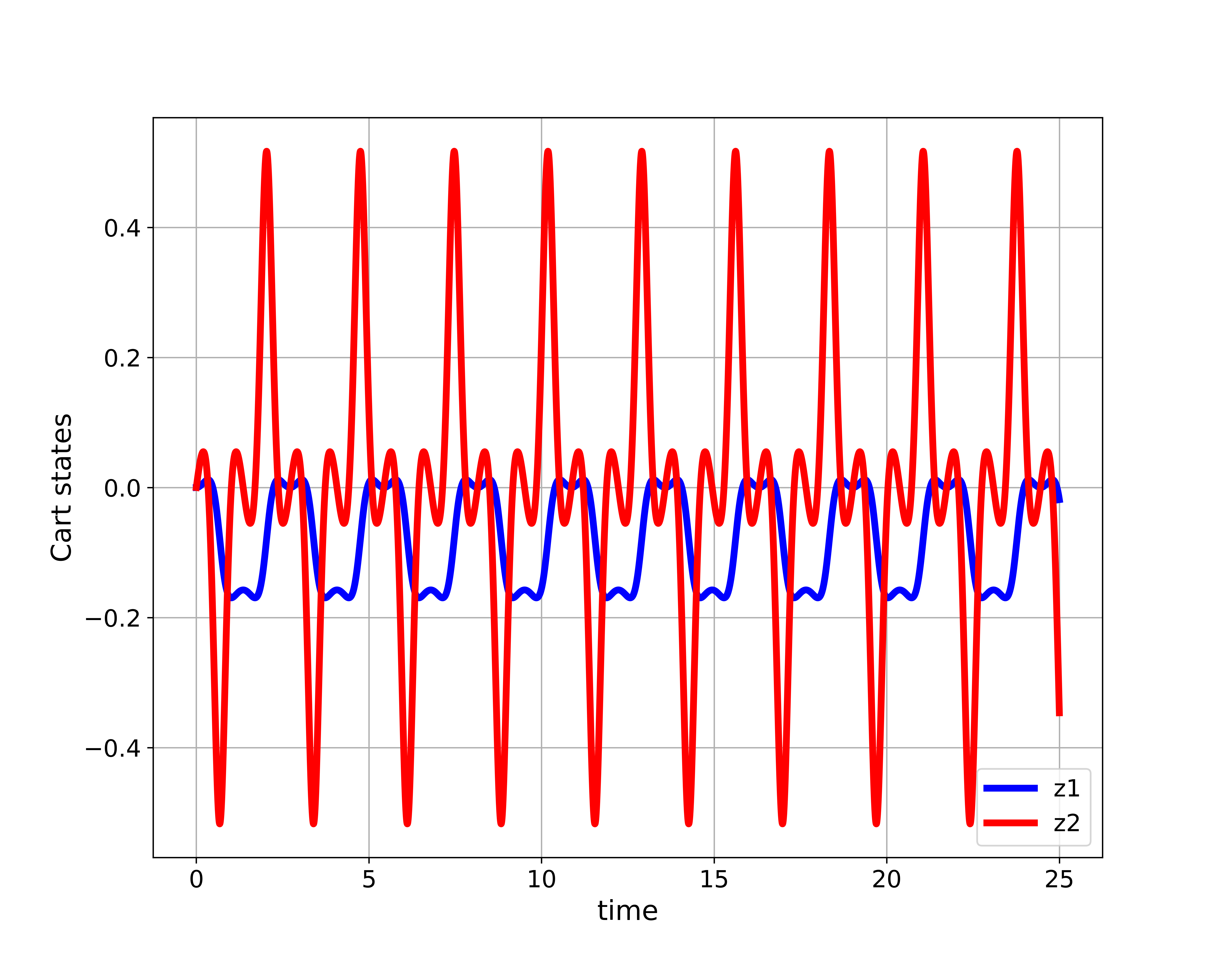
Next, we define the time vector for simulation and the control force time sequence. Finally, we define the initial condition for simulation, and we simulate the state-space model by using the function “odeint()”. The first input argument is the previously defined function defining the state-space model “stateSpaceModel”. The second input argument is the initial state “initialState”. The third input argument is the simulation time vector denoted by “simulationTime”. The final input argument is a tuple consisting of the time sequence and input force vector. Finally, we save the generated simulation data, and we plot the state trajectories. The state trajectories are given below.
 and ).
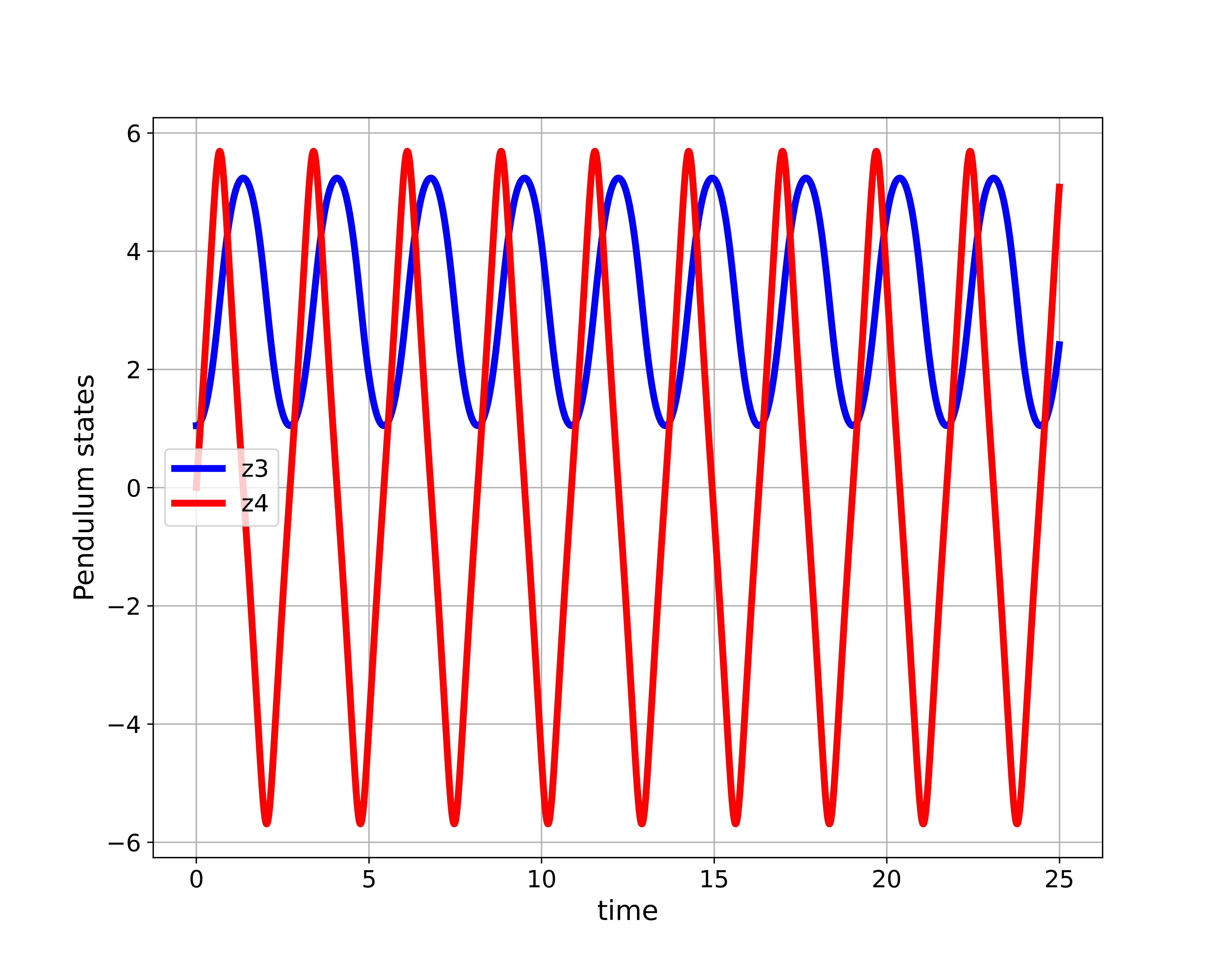
 and ).