What is Importance Sampling? – Detailed Explanation with Python Implementation and Simulation – Fusion of Engineering, Control, Coding, Machine Learning, and Science

In this Python, statistics, estimation, and mathematics tutorial, we introduce the concept of importance sampling. The importance sampling method is a Monte Carlo method for approximately computing expectations and integrals of functions of random variables. The importance sampling method is extensively used in computational physics, Bayesian estimation, machine learning, and particle filters for state estimation of dynamical systems. For us, the most interesting application is particle filters for state estimation of dynamical systems. This topic will be covered in our future tutorials. For the time being it is of paramount importance to properly explain the importance sampling method. Besides explaining the importance sampling method, in this tutorial, we also explain how to implement the importance sampling method in Python and its SciPy library. The YouTube tutorial accompanying this webpage is given below.

Basics of Importance Sampling Method

In our previous tutorial, whose link is given here, we explained how to approximate the integrals of functions of random variables by using the basic Monte Carlo method. Briefly speaking, the problem is to approximately compute the integral

(1) $\begin{align*}I=\int_{a}^{b}g(x)f(x)\text{d}x\end{align*}$

where $X$ is a random variable, $f(x)$ is the probability density function of the random variable $x$ , and $g(x)$ is a nonlinear function. The real numbers of $a$ and $b$ are integration bounds (they can also be equal to plus or minus infinity $\infity$ ). This integral can also be seen as the expectation of the random variable $g(X)$ :

(2) $\begin{align*}I=\mathbb{E}[g(x)]=\int_{a}^{b}g(x)f(x)\text{d}x\end{align*}$

The Monte Carlo method approximates this integral by performing the following two steps:

Draw $N$ random samples of $X$ from the distribution described by $f(x)$ . Let these samples be denoted by $x_{1},x_{2},x_{3},\ldots, x_{N}$ .
Approximate the integral by the following expression
(3) $\begin{align*}\hat{I}_{N}=\frac{1}{N}\sum_{i=1}^{N}g(x_{i})\end{align*}$

where $\hat{I}_{N}$ is the approximation of the integral (2) by using $N$ random samples of $X$ .

The above-described Monte Carlo method makes an assumption that it is possible to draw samples from the distribution described by $f(x)$ . Now, in a number of scenarios it might either be impossible or very difficult to draw samples from the distribution $f(x)$ . Also, even if it is possible to draw samples from this distribution, it might be preferable to draw samples from some other distribution.

We would like to draw samples from some other distribution and use this distribution to approximate the integral (1). How to do that? Let $q(x)$ be a probability density function of a new distribution we can easily draw samples from (we will later on give a special name to this distribution). Then, we can transform the integral as follows

(4) $\begin{align*}I=\int_{a}^{b}g(x)f(x)\text{d}x=\int_{a}^{b}g(x)\frac{f(x)}{q(x)}q(x)\text{d}x\end{align*}$

By introducing a new variable (later on, we will introduce a name for this variable):

(5) $\begin{align*}w(x)=\frac{f(x)}{q(x)}\end{align*}$

The integral (4) can be written as follows

(6) $\begin{align*}I=\int_{a}^{b}w(x)g(x)q(x)\text{d}x\end{align*}$

The last integral can be seen as an expectation of the nonlinear function $w(x)g(x)$ :

(7) $\begin{align*}I=\mathbb{E}[w(x)g(x)]=\int_{a}^{b}w(x)g(x)q(x)\text{d}x\end{align*}$

Consequently, we can use the Monte Carlo method to approximate this integral:

(8) $\begin{align*}\hat{I}_{N}=\frac{1}{N}\sum_{i=1}^{N} w(x_{i})g(x_{i})\end{align*}$

where $x_{i}$ , $i=1,2,3,\ldots,N$ , are the samples of $X$ drawn from the new distribution $q(x)$ , and where

(9) $\begin{align*}w(x_{i})=\frac{f(x_{i})}{q(x_{i})}\end{align*}$

The approximation (8) is the importance sampling approximation of the original integral (1). It can be shown that as $N$ approaches infinity, the approximation approaches the exact value of the integral. Furthermore, the importance sampling approximation is an unbiased estimator of the exact value of the integral.

Next, we introduce the following names and terminology

The function $q(x)$ is called the proposal density or the importance (sampling) density. Other names for this function are the proposal function or the importance function. We have complete freedom to select this function. However, this function has to satisfy several requirements. First of all, it needs to satisfy the following requirement
(10) $\begin{align*}f(x)>0 => q(x)>0,\;\; \forall x\end{align*}$

That is, $f(x)$ and $q(x)$ need to have the same support. Then, we should be able to easily draw samples from $q(x)$ . Ideally, we would like $q(x)$ to have a similar shape to $f(x)$ . Also, in order to minimize the Monte Carlo estimator variance, we would like to select $q(x)$ to be proportional to $|g(x)|f(x)$ . In practice, we often cannot select $q(x)$ to satisfy all the ideal requirements, and we need to make a trade-off. We often need to try several different forms of $q(x)$ .
The parameters $w(x_{i})$ defined in (9) are called the importance weights. They are computed on the basis of the samples $x_{i}$ sampled from the proposal density $q(x)$ . The intuitive explanation of the importance weights is that they make a weighted adjustment of the Monte Carlo average. This adjustment takes into account the fact that we are sampling from $q(x)$ instead of sampling from $f(x)$ .

Since this is an introduction-level tutorial on the importance sampling, we will not discuss other theoretical properties of the importance sampling method. We will talk more about the importance sampling method in our tutorial on particle filters. Instead, in the sequel, we explain how to simulate the importance sampling method in Python.

Importance Sampling Method in Python

Here, we consider a test case. We consider a problem of computing the mean of a normal distribution. This problem is to compute the following expectation integral

(11) $\begin{align*}I=\mathbb{E}[X]=\int_{-\infty}^{+\infty} x f(x)\text{d}x\end{align*}$

where $f(x)$ is a probability density function of the normal distribution. Let us assume that the mean of $f(x)$ is $\mu_{f}=10$ , and that the standard deviation is $\sigma_{f}=5$ . However, let us additionally assume that we cannot draw samples from this distribution. Instead, let us assume that we can only draw samples from another normal distribution denoted by $q(x)$ . The mean of $q(x)$ is $\mu_{q}=0$ and the standard deviation is $\sigma_{q}=6$ . The normal distribution $q(x)$ is the proposal distribution. The importance sampling approximation of the integral (11) is

(12) $\begin{align*}\hat{I}_{N}=\frac{1}{N}\sum_{i=1}^{N} w(x_{i})x_{i}\end{align*}$

where $x_{i}$ , $i=1,2,3,\ldots, N$ are random samples of $X$ sampled from the proposal distribution $q(x)$ , and the importance weights are defined as

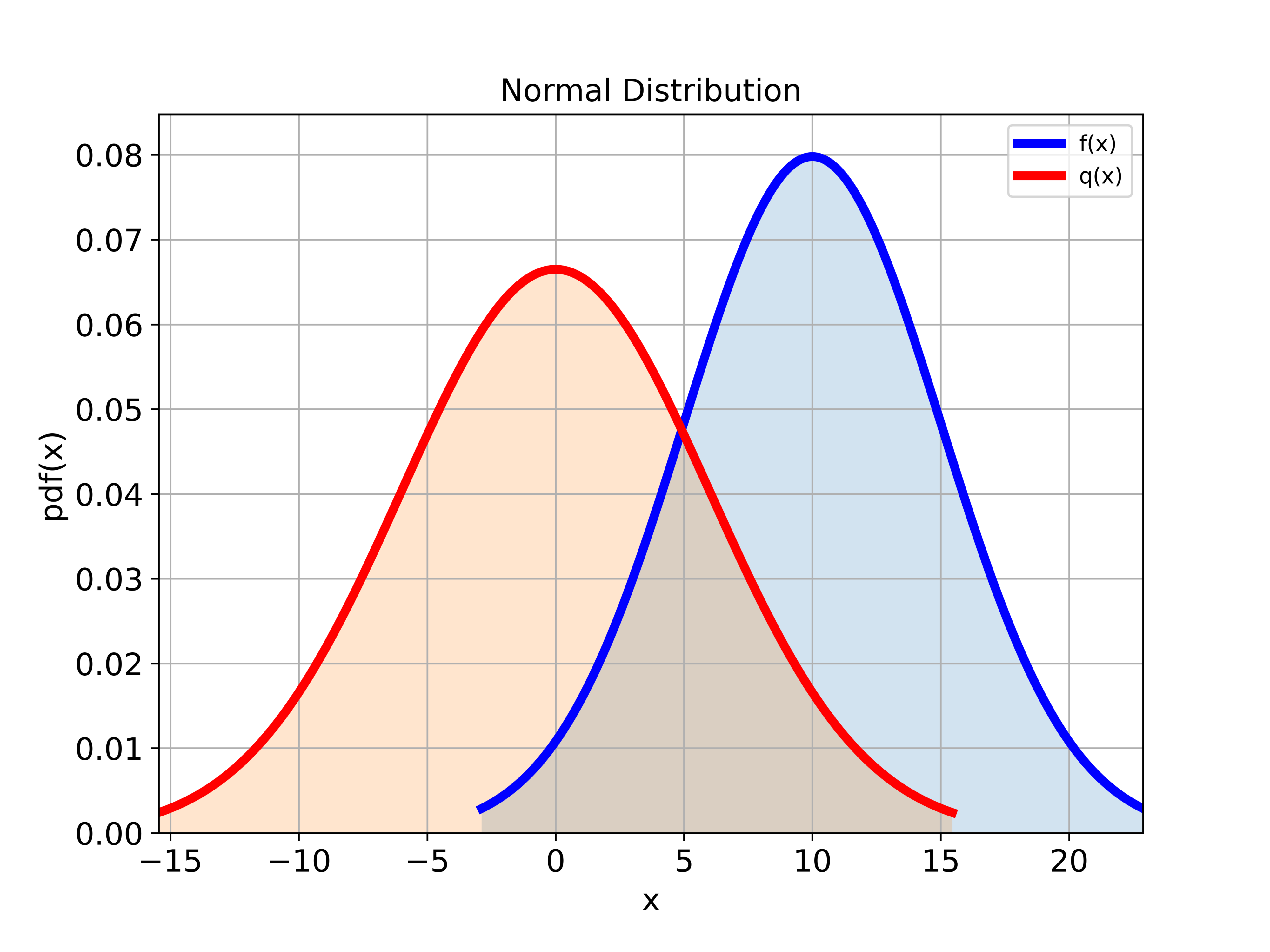
(13) $\begin{align*}w(x_{i})=\frac{f(x_{i})}{q(x_{i})}\end{align*}$

In our previous tutorials, given here, and here, we explained how to construct normal distributions in Python and how to draw samples from normal distributions. Consequently, to understand the Python script given below, we suggest that you go over these two tutorials. First, we create the two distributions in Python and SciPy and plot them:

import numpy as np
from scipy import stats
import matplotlib.pyplot as plt

# define the f and q normal distributions in Python:

# mean value
meanValueF=10
meanValueQ=0

# standard deviation
standardDeviationF=5
standardDeviationQ=6

# create normal distributions 
distributionF=stats.norm(loc=meanValueF, scale=standardDeviationF)
distributionQ=stats.norm(loc=meanValueQ, scale=standardDeviationQ)

# plot the probability density functions of two distributions
startPointXaxisF=distributionF.ppf(0.005)
endPointXaxisF=distributionF.ppf(0.995)
xValueF = np.linspace(startPointXaxisF,endPointXaxisF, 500)
yValueF = distributionF.pdf(xValueF)

startPointXaxisQ=distributionQ.ppf(0.005)
endPointXaxisQ=distributionQ.ppf(0.995)
xValueQ = np.linspace(startPointXaxisQ,endPointXaxisQ, 500)
yValueQ = distributionQ.pdf(xValueQ)


# plot the probability density function
plt.figure(figsize=(8,6))
plt.gca()  
plt.plot(xValueF,yValueF, color='blue',linewidth=4, label='f(x)')
plt.fill_between(xValueF, yValueF, alpha=0.2)

plt.plot(xValueQ,yValueQ, color='red',linewidth=4, label='q(x)')
plt.fill_between(xValueQ, yValueQ, alpha=0.2)
plt.title('Normal Distribution', fontsize=14)
plt.xlabel('x', fontsize=14)
plt.ylabel('pdf(x)',fontsize=14)
plt.tick_params(axis='both',which='major',labelsize=14)
plt.grid(visible=True)
plt.xlim((startPointXaxisQ,endPointXaxisF)) 
plt.ylim((0,max(yValueF)+0.005))
plt.legend() 
plt.savefig('normalDistribution2.png',dpi=600)
plt.show()

The graph is shown in the figure below.

The following Python script implements the importance sampling method and the estimator equation (12)



# generate random samples from the normal distribution and compute the mean
sampleSize1=100
randomSamples1 = distributionQ.rvs(size=sampleSize1)
# compute the terms 
listTerms1=[(distributionF.pdf(xi)/distributionQ.pdf(xi))*xi for xi in randomSamples1]
estimate1=np.array(listTerms1).mean()



# generate random samples from the normal distribution and compute the mean
sampleSize2=10000
randomSamples2 = distributionQ.rvs(size=sampleSize2)
# compute the terms 
listTerms2=[(distributionF.pdf(xi)/distributionQ.pdf(xi))*xi for xi in randomSamples2]
estimate2=np.array(listTerms2).mean()

As the result, we obtain

estimate1=11.637370568072074
estimate2=10.483881203350437

As the number of samples increases, we can observe that the importance sampling estimate approaches the exact value of the mean of the distribution $f(x)$ , that is, it approaches 10. That is, the variance of the estimator decreases with the increase of the number of samples.

Basics of Importance Sampling Method

Importance Sampling Method in Python

admin

You might also like

State-Space Modeling of Double Mass-Spring-Damper System with Python Modeling

Correct Explanation of State Observers for State Estimation of State-Space Models with Python Simulations

How to Set or Adjust the Figure Size in Python and Matplotlib