State-Space Modeling of Double Mass-Spring-Damper System with Python Modeling – Fusion of Engineering, Control, Coding, Machine Learning, and Science

In this dynamical systems, control engineering, and control theory tutorial, we develop a state-space model of a double mass-spring-damper system. We also explain how to simulate the derived state-space model in Python. We use two approaches for discretizing the model of the mass-spring-damper system. The first approach is based on the Backward Euler method and the second approach is based on the Python Control Systems Library. The main motivation for creating this video tutorial comes from the fact that mass-spring-damper systems are prototypical and generic systems that can represent physical models of a large number of dynamical systems, such as car suspension systems, harmonic oscillators, robotic arms, etc.

State-Space Model of Double Mass-Spring-Damper System

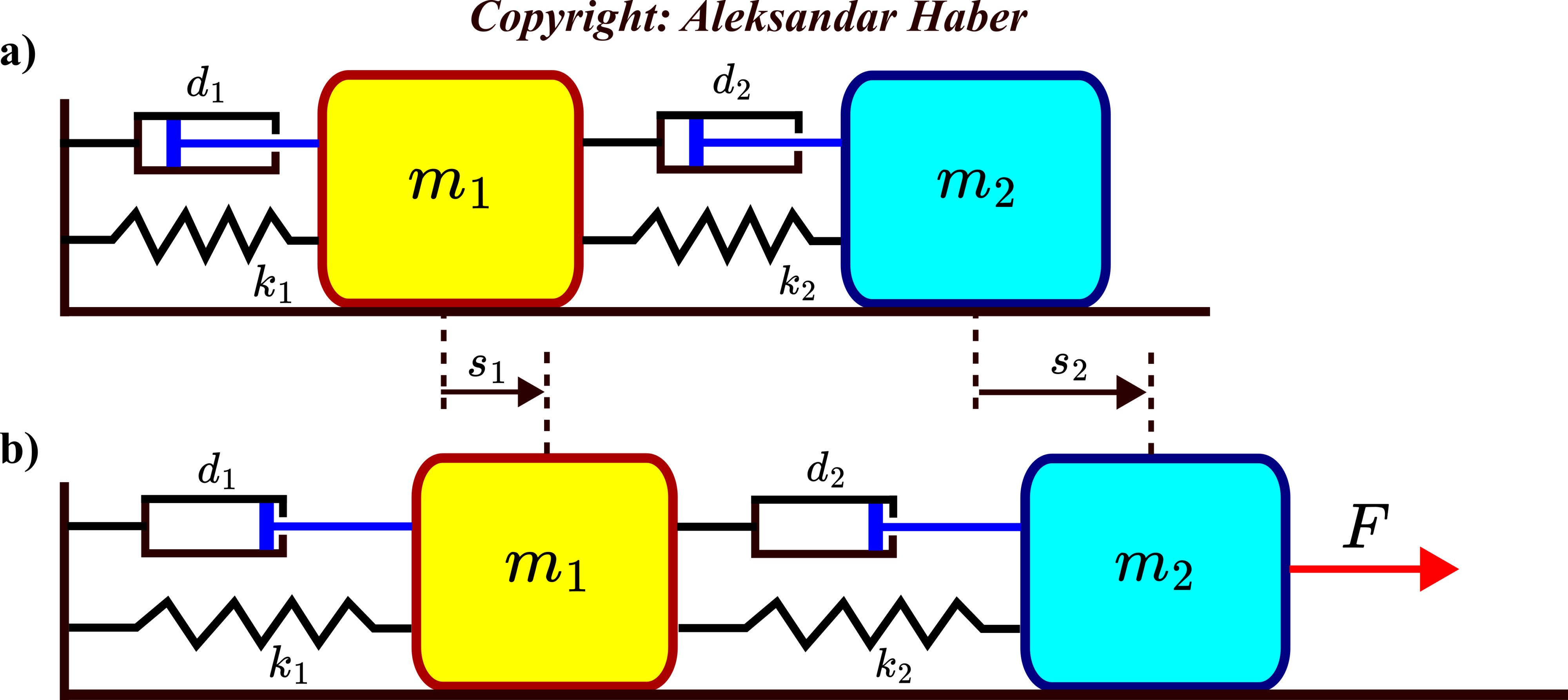
The double-mass-spring damper system is shown in the figure below.

Figure 1: Double mass-spring damper system. (a) The system configuration in its equilibrium position. (b) The configuration of the system after the force $F$ is applied.

The system consists of two objects with masses of $m_{1}$ and $m_{2}$ . The objects are connected by springs and dampers. The spring constants of the first and second springs are $k_{1}$ and $k_{2}$ , respectively. The damping constants of the first and second dampers are $d_{1}$ and $d_{2}$ , respectively. In Fig. 1(a), the system is shown in its equilibrium configuration without external forces. In Fig.1(b), the force $F$ is applied to the second object. Due to the action of this force, both objects are displaced from their equilibrium positions. The displacements from the equilibrium points for the first and second objects are denoted by $s_{1}$ and $s_{2}$ , respectively. The velocities of the first and second objects are denoted by $\dot{s}_{1}$ and $\dot{s}_{2}$ . The accelerations of the first and second objects are denoted by $\ddot{s}_{1}$ and $\ddot{s}_{2}$ .

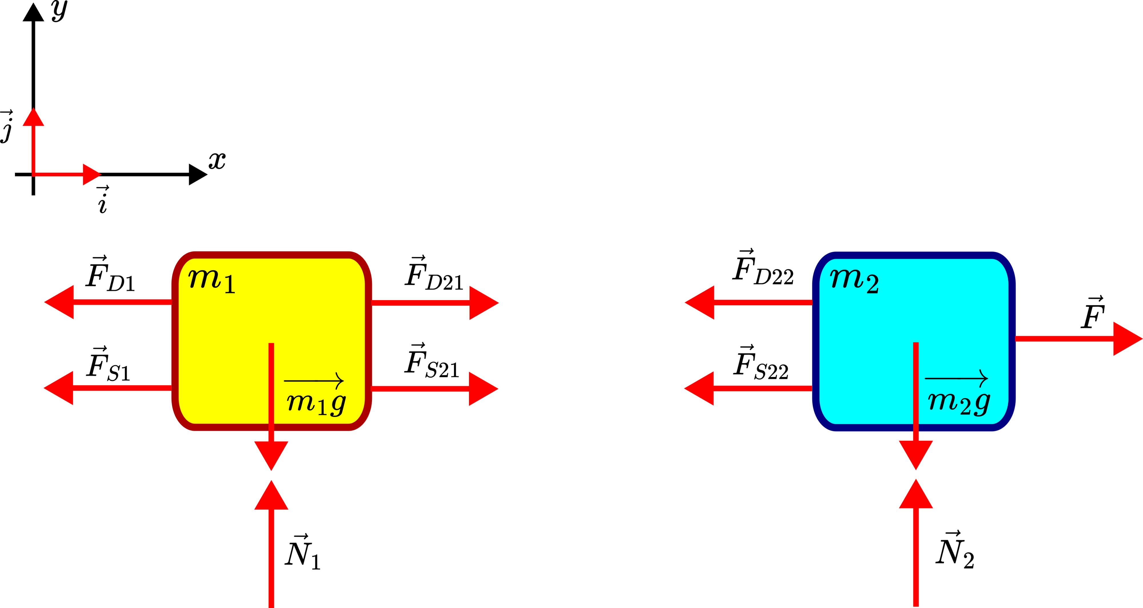
Our main goal is to develop a state-space model of this system. For that purpose, we need to construct a free-body diagram of the system. The free-body diagram is shown in the figure below.

We assume that the friction between objects and the supporting surface can be neglected. Also, we assume that the masses of springs and dampers are much smaller than the object masses. Consequently, we neglect the masses of springs and dampers.

Figure 2 above shows the free-body diagram of the system. Here is the explanation of the vectors and forces in the free-body diagram

$\vec{i}$ and $\vec{j}$ are unit vectors of the $x$ and $y$ axes.
$\vec{F}_{S1}$ is the force that the spring 1 is exerting on the object 1. This force is given by
(1) $\begin{align*}\vec{F}_{S1}=-k_{1}s_{1}\vec{i}\end{align*}$
The force $\vec{F}_{D1}$ is the force that the damper 1 is exerting on the object 1. This force is given by
(2) $\begin{align*}\vec{F}_{D1}=-d_{1}\dot{s}_{1}\vec{i}\end{align*}$
The force $\vec{N}_{1}$ is the surface reaction force exerted on the object 1.
$\overrightarrow{m_{1}g}$ is the weight of the object 1.
The force $\vec{F}_{S21}$ is the force that the spring 2 is exerting on the object 1. This force is given by
(3) $\begin{align*}\vec{F}_{S21}=k_{2}(s_{2}-s_{1})\vec{i}\end{align*}$
The force $\vec{F}_{D21}$ is the force that the damper 2 is exerting on the object 1. This force is given by
(4) $\begin{align*}\vec{F}_{D21}=d_{2}(\dot{s}_{2}-\dot{s}_{1})\vec{i}\end{align*}$
The force $\vec{F}_{S22}$ is the force that the spring 2 is exerting on the object 2.
The force $\vec{F}_{D22}$ is the force that the damper 2 is exerting on the object 2.

Due to the fact that the masses of springs and dampers can be neglected, we have

(5) $\begin{align*}\vec{F}_{S21}&=-\vec{F}_{S22} \\\vec{F}_{D21}&=-\vec{F}_{D22}\end{align*}$

From these two equations, we obtain

(6) $\begin{align*}\vec{F}_{S22}= - k_{2}(s_{2}-s_{1})\vec{i} \\\vec{F}_{D22}= - d_{2}(\dot{s}_{2}-\dot{s}_{1})\vec{i}\end{align*}$

From the second Newton’s law, we have

(7) $\begin{align*}m_{1}\vec{a}_{1}&=\vec{F}_{D1}+\vec{F}_{S1}+\overrightarrow{m_{1}g}+\vec{N}_{1}+\vec{F}_{D21}+\vec{F}_{S21} \\m_{2}\vec{a}_{2}&=\vec{F}_{D22}+\vec{F}_{S22}+\overrightarrow{m_{2}g}+\vec{N}_{2}+\vec{F}\end{align*}$

where $\vec{a}_{1}$ and $\vec{a}_{2}$ are accelerations of the first and second objects, respectively. By using (1)-(6) and by projecting the last two equations onto the horizontal $x$ axis, we obtain the following two equations:

(8) $\begin{align*}m_{1}\ddot{s}_{1} & = -d_{1}\dot{s}_{1}-k_{1}s_{1}+d_{2}(\dot{s}_{2}-\dot{s}_{1})+k_{2}(s_{2}-s_{1}) \\m_{2}\ddot{s}_{2} & = - d_{2}(\dot{s}_{2}-\dot{s}_{1})-k_{2}(s_{2}-s_{1})+F \end{align*}$

The last two equations can be written as follows

(9) $\begin{align*}m_{1}\ddot{s}_{1} & =-(k_{1}+k_{2})s_{1}-(d_{1}+d_{2}) \dot{s}_{1} +k_{2}s_{2}+d_{2}\dot{s}_{2} \\m_{2}\ddot{s}_{2} & =k_{2}s_{1} + d_{2}\dot{s}_{1}-k_{2}s_{2} - d_{2}\dot{s}_{2}+F \end{align*}$

Then, we introduce the state-space variables

(10) $\begin{align*}x_{1}=s_{1},\;\; x_{2}=\dot{s}_{1}, \;\; x_{3}=s_{2},\;\; x_{4}=\dot{s}_{2} \end{align*}$

By using these state space variables, we can write the equations (9) as follows

(11) $\begin{align*}\dot{x}_{1}&=x_{2} \\m_{1}\dot{x}_{2}&=-(k_{1}+k_{2})x_{1}-(d_{1}+d_{2})x_{2}+k_{2}x_{3}+d_{2}x_{4} \\\dot{x}_{3}&=x_{4} \\m_{2}\dot{x}_{4} & =k_{2}x_{1} + d_{2}x_{2}-k_{2}x_{3} - d_{2}x_{4}+F \end{align*}$

From the last system of differential equations, we obtain

(12) $\begin{align*}\dot{x}_{1}&=x_{2} \\\dot{x}_{2}&=-\frac{k_{1}+k_{2}}{m_{1}}x_{1}-\frac{d_{1}+d_{2}}{m_{1}}x_{2}+\frac{k_{2}}{m_{1}}x_{3}+\frac{d_{2}}{m_{1}}x_{4} \\\dot{x}_{3}&=x_{4} \\\dot{x}_{4} & =\frac{k_{2}}{m_{2}}x_{1} + \frac{d_{2}}{m_{2}}x_{2}-\frac{k_{2}}{m_{2}}x_{3} - \frac{d_{2}}{m_{2}}x_{4}+\frac{1}{m_{2}}F \end{align*}$

The system of equations (12) can be written in the state-space form:

(13) $\begin{align*}\begin{bmatrix}\dot{x}_{1} \\ \dot{x}_{2} \\ \dot{x}_{3} \\ \dot{x}_{4}\end{bmatrix}= \begin{bmatrix} 0 & 1 & 0 & 0 \\ -\frac{k_{1}+k_{2}}{m_{1}} & -\frac{d_{1}+d_{2}}{m_{1}} & \frac{k_{2}}{m_{1}} & \frac{d_{2}}{m_{1}} \\ 0 & 0 & 0 & 1 \\ \frac{k_{2}}{m_{2}} & \frac{d_{2}}{m_{2}} & -\frac{k_{2}}{m_{2}} & -\frac{d_{2}}{m_{2}} \end{bmatrix}\begin{bmatrix}x_{1} \\ x_{2} \\ x_{3} \\ x_{4}\end{bmatrix}+\begin{bmatrix} 0 \\ 0 \\ 0 \\ \frac{1}{m{2}} \end{bmatrix}F \end{align*}$

We assume that only the position of the first object can be directly observed. This can be achieved by using a distance sensor. Under this assumption, the output equation has the following form

(14) $\begin{align*}\mathbf{y}=\begin{bmatrix}1 & 0 & 0 & 0\end{bmatrix}\begin{bmatrix} x_{1} \\ x_{2} \\ x_{3} \\ x_{4} \end{bmatrix}\end{align*}$

The state equation (13) and the output equation (14) can be written compactly as follows

(15) $\begin{align*}\dot{\mathbf{x}} & =A\mathbf{x}+B\mathbf{u} \\\mathbf{y}& = C\mathbf{x}\end{align*}$

where

(16) $\begin{align*}& \mathbf{x}=\begin{bmatrix}x_{1} \\ x_{2} \\ x_{3} \\ x_{4}\end{bmatrix},\; \mathbf{u}=\begin{bmatrix}F \end{bmatrix},\;\; A=\begin{bmatrix} 0 & 1 & 0 & 0 \\ -\frac{k_{1}+k_{2}}{m_{1}} & -\frac{d_{1}+d_{2}}{m_{1}} & \frac{k_{2}}{m_{1}} & \frac{d_{2}}{m_{1}} \\ 0 & 0 & 0 & 1 \\ \frac{k_{2}}{m_{2}} & \frac{d_{2}}{m_{2}} & -\frac{k_{2}}{m_{2}} & -\frac{d_{2}}{m_{2}} \end{bmatrix},\;\; \\ & B=\begin{bmatrix} 0 \\ 0 \\ 0 \\ \frac{1}{m_{2}} \end{bmatrix},\;\; C=\begin{bmatrix}1 & 0 & 0 & 0 \end{bmatrix}\end{align*}$

We will use two approaches for simulating the state-space model in Python. The first approach is based on the discretization of the model by using the Backward Euler method. The second approach for simulation is based on the Control Systems Toolbox.

Simulation of State-Space Model in Python: Discretize the Model Using Backward Euler Method

Due to its simplicity and good stability properties, we use the Backward Euler method to perform the discretization of the state-space model (15). This method approximates the state derivative as follows

(17) $\begin{align*}\dot{\mathbf{x}}\approx \frac{\mathbf{x}_{k}-\mathbf{x}_{k-1}}{h}\end{align*}$

where $\mathbf{x}_{k}=\mathbf{x}(kh)$ , $h$ is a discretization constant, and $k=0,1,2,\ldots$ is a discrete-time instant. By substituting this approximation in (15), we obtain:

(18) $\begin{align*}\frac{\mathbf{x}_{k}-\mathbf{x}_{k-1}}{h}=A\mathbf{x}_{k}+B\mathbf{u}_{k-1}\end{align*}$

For simplicity, we assumed that the discrete-time index of the input is $k-1$ . We can also assume that the discrete-time index of input is $k$ if we want. However, then, when simulating the system dynamics we will start from $k=1$ . From the last equation, we have

(19) $\begin{align*}\mathbf{x}_{k}-\mathbf{x}_{k-1}&=hA\mathbf{x}_{k}+hB\mathbf{u}_{k-1} \\\mathbf{x}_{k}-hA\mathbf{x}_{k}&=\mathbf{x}_{k-1}+hB\mathbf{u}_{k-1} \\\big(I- hA \big) \mathbf{x}_{k}& =\mathbf{x}_{k-1}+hB\mathbf{u}_{k-1} \\\mathbf{x}_{k}& =\big(I- hA \big)^{-1}\mathbf{x}_{k-1}+h\big(I- hA \big)^{-1} B\mathbf{u}_{k-1} \end{align*}$

The last equation can be written compactly as follows

(20) $\begin{align*}\mathbf{x}_{k}=A_{D}\mathbf{x}_{k-1}+B_{D} \mathbf{u}_{k-1}\end{align*}$

where

(21) $\begin{align*}A_{D}=(I-hA)^{-1},\;\; B_{D}=hA_{D}B\end{align*}$

On the other hand, the output equation remains unchanged

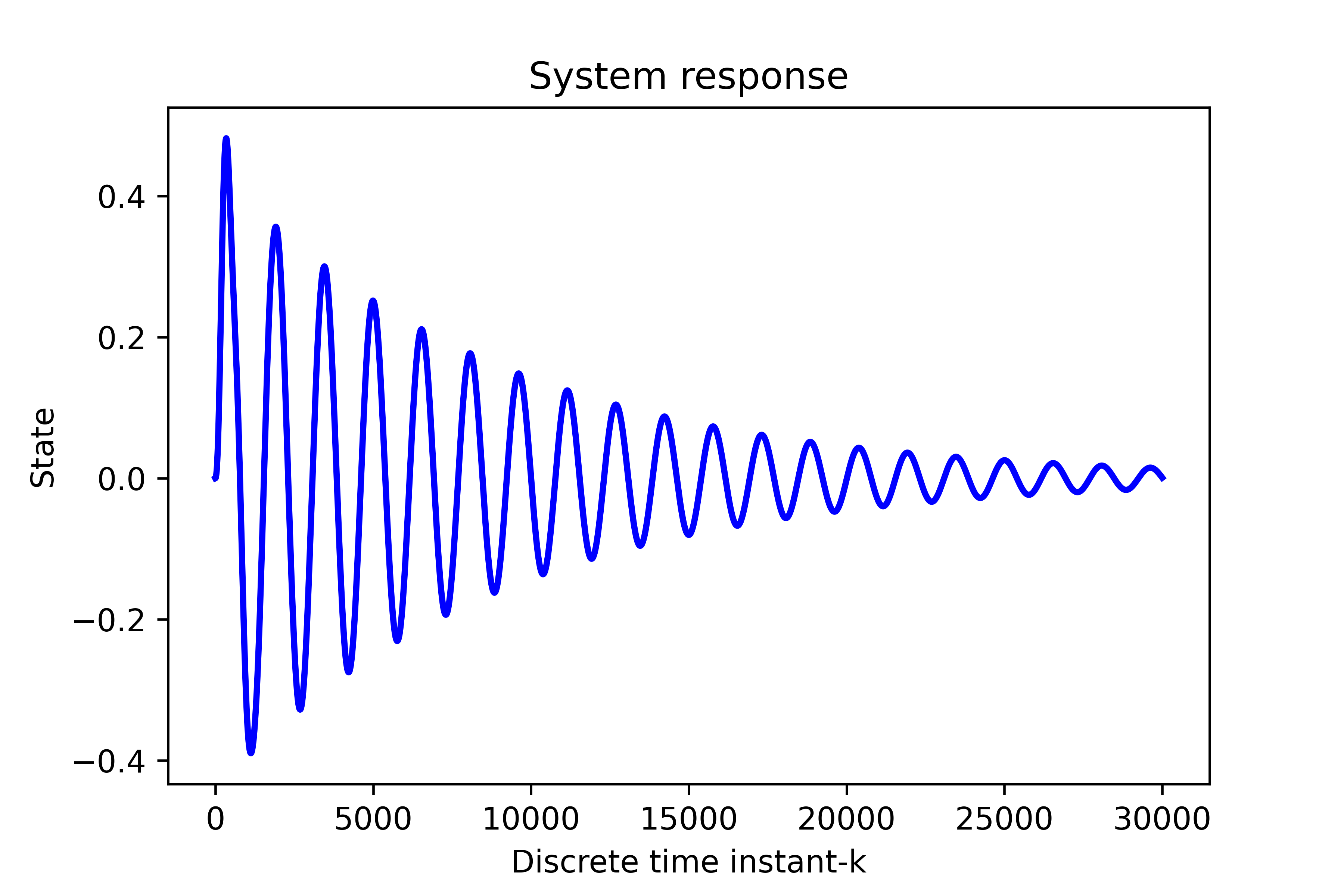
(22) $\begin{align*}\mathbf{y}_{k}=C\mathbf{x}_{k}\end{align*}$

In the sequel, we present a Python script for discretizing the system and computing the system response to the control input signals. The Python script is given below. We simulate the scaled step response.

import numpy as np
import matplotlib.pyplot as plt
from numpy.linalg import inv
 
# define the system parameters
m1=2  ; m2=3   ; k1=100  ; k2=200 ; d1=1  ; d2=5; 
 
 # define the continuous-time system matrices
A=np.array([[0, 1, 0, 0],
             [-(k1+k2)/m1 ,  -(d1+d2)/m1 , k2/m1 , d2/m1 ], 
             [0 , 0 ,  0 , 1], 
             [k2/m2,  d2/m2, -k2/m2, -d2/m2]])
B=np.array([[0],[0],[0],[1/m2]])
C=np.array([[1, 0, 0, 0]])
 
#define an initial state for simulation
x0=np.zeros(shape=(4,1))
 
# define the number of time-samples used for the simulation 
time=30000
# discretization constant
h=0.001
#define an input sequence for the simulation
#input_seq=np.random.rand(time,1)
input_seq=10*np.ones(shape=(1,time))
#plt.plot(input_sequence)
 
I=np.identity(A.shape[0]) # this is an identity matrix
A_D=inv(I-h*A)
B_D=h*np.matmul(A_D,B)
C_D=C 
 
# check the eigenvalues
# continuous time system
eigen_A=np.linalg.eig(A)[0]
# discrete-time system
print(eigen_A)
eigen_A_D=np.linalg.eig(A_D)[0]
# the following function simulates the state-space model using 
# the backward Euler method
# the input parameters are:
#    -- Am,Bm,Cm           - discrete-time system matrices 
#    -- initial_state      - the initial state of the system 
#    -- input_sequence     - input sequence for simulation
#    -- time_steps         - the total number of simulation time steps 
# this function returns the state sequence and the output sequence
# they are stored in the matrices Xm and Ym, respectively
def simulate(Am,Bm,Cm,initial_state,input_sequence,time_steps):
    Xm=np.zeros(shape=(Am.shape[0],time_steps+1))
    Ym=np.zeros(shape=(Cm.shape[0],time_steps+1))
     
    for i in range(0,time_steps):
       if i==0:
           Xm[:,[i]]=initial_state
           Ym[:,[i]]=np.matmul(Cm,initial_state)
           inputTmp=input_sequence[0,i].reshape(Bm.shape[1],1)
           x=np.matmul(Am,initial_state)+np.matmul(Bm,inputTmp)
       else:
           Xm[:,[i]]=x
           Ym[:,[i]]=np.matmul(Cm,x)
           inputTmp=input_sequence[0,i].reshape(Bm.shape[1],1)
           x=np.matmul(Am,x)+np.matmul(Bm,inputTmp)
    
    Xm[:,[-1]]=x
    Ym[:,[-1]]=np.matmul(Cm,x)
    return Xm, Ym
     
state,output=simulate(A_D,B_D,C_D,x0,input_seq, time)    
 
plt.plot(state[1,:], color='blue',linewidth=2)
plt.xlabel('Discrete time instant-k')
plt.ylabel('State')
plt.title('System response')
plt.savefig('step_responseEuler.png',dpi=600)
plt.show()
# save the simulation data
np.save('matrixStateEuler.npy', state)

The simulation graph is shown below.

Simulation of Double Mass-Spring-Damper System by Using Python Control System Library

We simulate the state-space dynamics by using the Python Control Systems Library. The code is given below.

"""
@author: Aleksandar Haber 
date: 2023
pip install slycot   # optional
pip install control
"""
import matplotlib.pyplot as plt
import control as ct
import numpy as np
# this function is used for plotting of responses 
# it generates a plot and saves the plot in a file 
# xAxisVector - time vector
# yAxisVector - response vector
# titleString - title of the plot
# stringXaxis - x axis label 
# stringYaxis - y axis label
# stringFileName - file name for saving the plot, usually png or pdf files
def plottingFunction(xAxisVector,
                     yAxisVector,
                     titleString,
                     stringXaxis,
                     stringYaxis,
                     stringFileName):
    
    plt.figure(figsize=(8,6))
    plt.plot(xAxisVector,yAxisVector, color='blue',linewidth=4)
    plt.title(titleString, fontsize=14)
    plt.xlabel(stringXaxis, fontsize=14)
    plt.ylabel(stringYaxis,fontsize=14)
    plt.tick_params(axis='both',which='major',labelsize=14)
    plt.grid(visible=True)
    plt.savefig(stringFileName,dpi=600)
    plt.show()
    
###############################################################################    
#                   Open-loop state-space model      
###############################################################################    
# define the system parameters
m1=2  ; m2=3   ; k1=100  ; k2=200 ; d1=1  ; d2=5; 
 
# define the continuous-time system matrices
A=np.array([[0, 1, 0, 0],
             [-(k1+k2)/m1 ,  -(d1+d2)/m1 , k2/m1 , d2/m1 ], 
             [0 , 0 ,  0 , 1], 
             [k2/m2,  d2/m2, -k2/m2, -d2/m2]])
B=np.array([[0],[0],[0],[1/m2]])
C=np.array([[1, 0, 0, 0]])
D=np.array([[0]])
 
#define an initial state for simulation
#x0=np.random.rand(2,1)
x0=np.zeros(shape=(4,1))
# define the state-space model
sysStateSpace=ct.ss(A,B,C,D)
# print the system
print(sysStateSpace)
###############################################################################
#            simulate the step response of the open-loop system 
###############################################################################
# define the time vector for simulation
startTime=0
numberSamples=30001
h=0.001
endTime=numberSamples*h
timeVector=np.linspace(startTime,endTime,numberSamples)
# define the control input vector for simulation
controlInputVector=10*np.ones(numberSamples)
# simulate the system 
# 1 input argument - state-space model 
# 2 input argument - time vector 
# 3 input argument - defined control input
# 4 input argument - initial state for simulation
returnSimulation = ct.forced_response(sysStateSpace,
                                      timeVector,
                                      controlInputVector,
                                      x0)
# outputs of the forced_response is the TimeResponseData 
# object consisting of 
# time values of returned objects     
returnSimulation.time
# computed outputs of the system 
returnSimulation.outputs
# state sequence of the system
returnSimulation.states 
# inputs used for simulation
returnSimulation.inputs 
# plot the simulation results 
plottingFunction(returnSimulation.time,
                 returnSimulation.states[1,:],
                 titleString='State',
                 stringXaxis='time [s]' , 
                 stringYaxis='State',
                 stringFileName='stateResponseSS.png')
# save the simulation data
np.save('matrixStateToolbox.npy', returnSimulation.states)

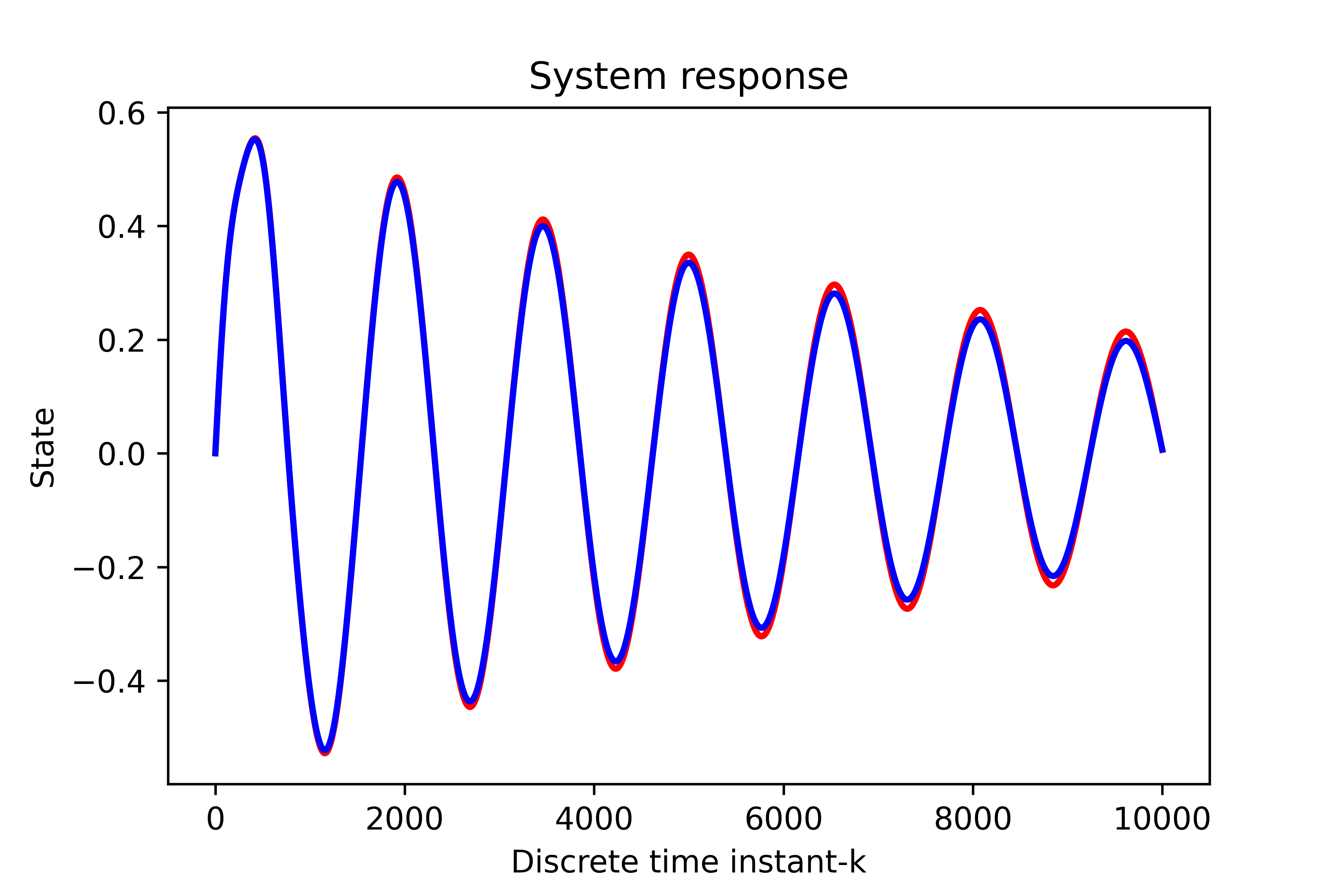
Comparison Between Backward Euler and Python Control Systems Library Toolbox

The following Python script compares two implementations.

import numpy as np
import matplotlib.pyplot as plt
loadedStateToolbox = np.load('matrixStateToolbox.npy')
loadedStateEuler=np.load('matrixStateEuler.npy')
plt.plot(loadedStateToolbox[3,0:10000], color='red',linewidth=2)
plt.plot(loadedStateEuler[3,0:10000], color='blue',linewidth=2)
plt.xlabel('Discrete time instant-k')
plt.ylabel('State')
plt.title('System response')
plt.savefig('comparions.png',dpi=600)
plt.show()

The comparison graph is given below.

State-Space Model of Double Mass-Spring-Damper System

Simulation of State-Space Model in Python: Discretize the Model Using Backward Euler Method

Simulation of Double Mass-Spring-Damper System by Using Python Control System Library

Comparison Between Backward Euler and Python Control Systems Library Toolbox

admin

You might also like

How to Draw Rectangles in OpenCV and Python

Symbolic Integration in Python by Using SymPy Library

Simple Discrete-time Model of Mobile Robot for Localization, SLAM, and Dead Reckoning