How To Approximate Expectations and Integrals of Functions by Using the Monte Carlo Method – Fusion of Engineering, Control, Coding, Machine Learning, and Science

In this mathematics and statistics tutorial, we explain one very important technique for approximating expectations and integrals of functions. This technique is based on the Monte Carlo Method. It is used in a large number of applications, such as simulation of random processes, state estimation of dynamical systems, machine learning, etc. For us, the most interesting application is state estimation of dynamical systems by using particle filters. Namely, the Monte Carlo method is the basis for the importance sampling method that serves as the basis of particle filters. The importance sampling is explained in the tutorial given here. In this tutorial, all the theoretical concepts are illustrated by using Python examples. The YouTube video accompanying this tutorial is given below.

Before we explain the main idea of the Monte Carlo method, we need to explain that this method is not only restricted to the approximation of expectations and integrals involving functions of random variables. As we explain in this tutorial, this method can also be used to approximate integrals of functions of deterministic variables.

Basic Idea of the Monte Carlo Method – Intro Example

Let us first consider a simple example. Let us say that we want to compute an expectation of a random scalar variable X with the probability density function $f(x)$ defined on the interval $x\in [a,b]$ (where $a$ and $b$ can also be plus or minus infinity):

(1) $\begin{align*}\mathbb{E}[X]=\int_{a}^{b}xf(x)\text{d}x\end{align*}$

where $\mathbb{E}[X]$ is the mathematical notation for the expectation operator. Let us now assume that the function $f(x)$ is such that this integral is difficult to exactly compute. Also, here we have to mention that everything explained in this tutorial can be generalized to the multidimensional case, that is when the random variable $X$ is a vector. In the multi-dimensional case, this integral might be even more difficult to compute. The main problem that we want to address is:

Knowing the mathematical form of the probability density function $f(x)$ , approximately compute the expectation (1).

The Monte Carlo method solves this problem in this way:

Draw $N$ random samples from the distribution described by $f(x)$ . Let these samples be denoted by $x_{1}, x_{2}, x_{3},\ldots, x_{N}$ .
Approximate the expectation by the following average:
(2) $\begin{align*}\hat{E}_{N}=\frac{1}{N}\sum_{i=1}^{N}x_{i}\end{align*}$

where $\hat{E}_{N}$ is an approximation of the expectation (1) computed by using $N$ samples of $X$ . The subscript $N$ in the notation $\hat{E}_{N}$ denotes the fact that the approximation is computed by using $N$ randomly drawn samples. The “hat” notation is usually used to denote an approximation or an estimate.

The equation (2) is called the Monte Carlo estimator of the expectation. From the law of large numbers, it follows that this estimator is a consistent estimator of expectation. Also, this estimator is unbiased. This means that

As $N$ approaches infinity, that is, when the number of random samples approaches infinity, the average (2) approaches the exact value of the expectation given by the equation (1).
For finite values of $N$ , if we draw $N$ samples a large number of times, and if we compute the average (2) for every set of $N$ samples, and if we compute an average of all averages (2), then this average will approximately be equal to the true value of expectation (1). Mathematically, this means that

(3) $\begin{align*}\mathbb{E}\big[ \hat{E}_{N} \big] =\mathbb{E}[X]\end{align*}$

Here it should be kept in mind that every time we draw $N$ random samples of $X$ , and compute the average $\hat{E}_{N}$ , the average will have a different value. This is because every set of $N$ samples will have different elements for different experiments of randomly selecting $N$ samples.

Before we generalize the Monte Carlo method to more complex functions and examples, let us now test this important method.

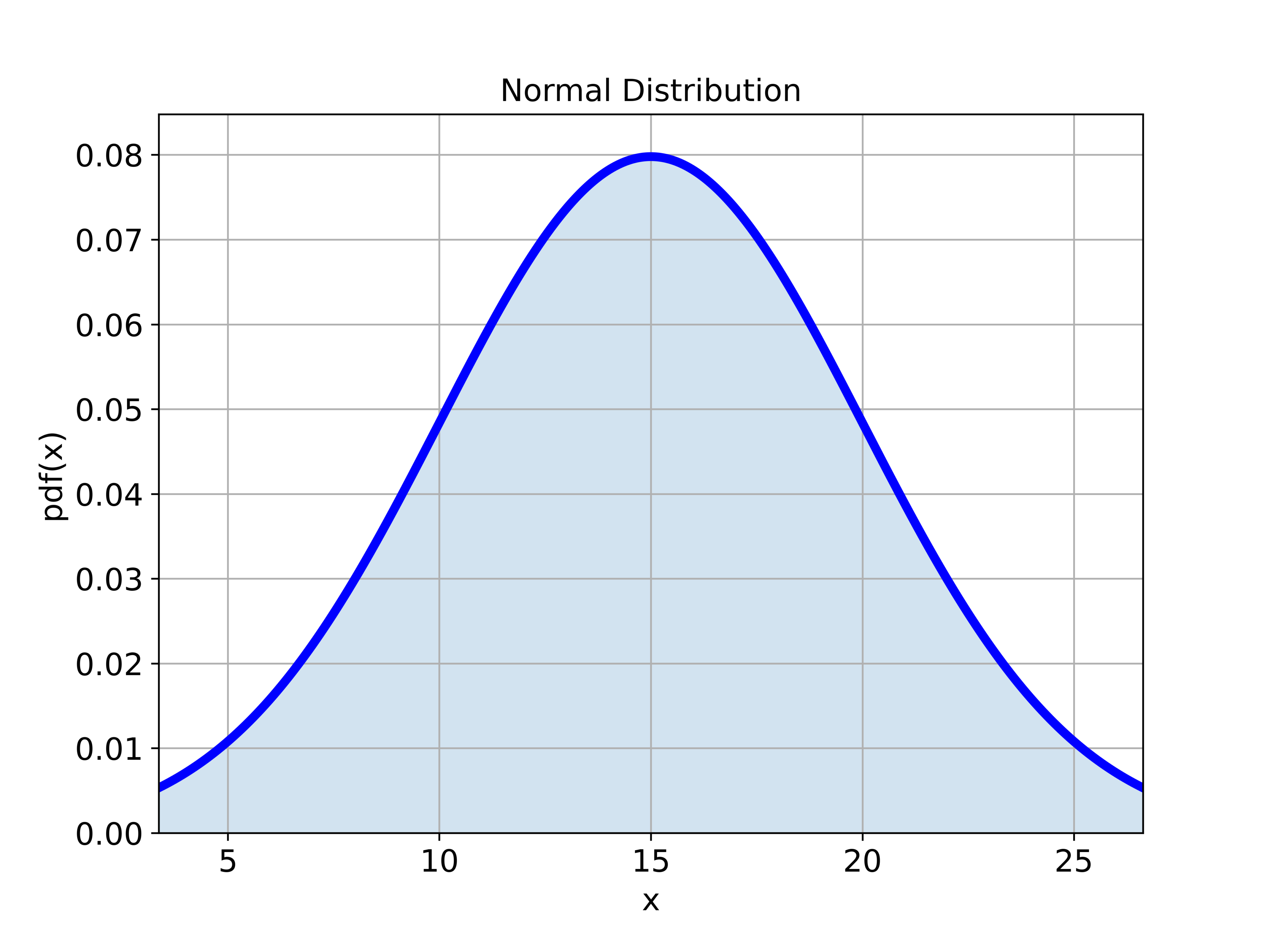
First, let us create a normal distribution in Python with a given mean and standard deviation. In our previous tutorial, given here and here, we explained how to construct a normal distribution in Python and how to draw samples from the normal distribution. By using these ideas, we construct a normal distribution in Python:

import numpy as np
from scipy import stats
import matplotlib.pyplot as plt

# define a normal distribution in Python:

# mean value
meanValue=15

# standard deviation
standardDeviation=5

# create a normal distribution 
# the keyword "loc" is used to specify the mean 
# the keyword "scale" is used to specify the standard deviation
distribution=stats.norm(loc=meanValue, scale=standardDeviation)

# plot the probability density function of the distribution
# start point
startPointXaxis=distribution.ppf(0.01)
# end point
endPointXaxis=distribution.ppf(0.99)

# create the x values
xValue = np.linspace(startPointXaxis,endPointXaxis, 500)

# the function pdf() will return the probability density function values
yValue = distribution.pdf(xValue)


# plot the probability density function
plt.figure(figsize=(8,6))
plt.gca()  
plt.plot(xValue,yValue, color='blue',linewidth=4)
plt.fill_between(xValue, yValue, alpha=0.2)
plt.title('Normal Distribution', fontsize=14)
plt.xlabel('x', fontsize=14)
plt.ylabel('pdf(x)',fontsize=14)
plt.tick_params(axis='both',which='major',labelsize=14)
plt.grid(visible=True)
plt.xlim((startPointXaxis,endPointXaxis)) 
plt.ylim((0,max(yValue)+0.005)) 
plt.savefig('normalDistribution2.png',dpi=600)
plt.show()

The distribution is shown in the figure below.

Next, let us draw samples of different sizes from this distribution, and let us compute the Monte Carlo estimator of the mean:

# generate random samples from the normal distribution and compute the mean
sampleSize1=10 
randomSamples1 = distribution.rvs(size=sampleSize1)


average1=randomSamples1.mean()

sampleSize2=20 
randomSamples2 = distribution.rvs(size=sampleSize2)


average2=randomSamples2.mean()

sampleSize3=40 
randomSamples3 = distribution.rvs(size=sampleSize3)


average3=randomSamples3.mean()

sampleSize4=100
randomSamples4 = distribution.rvs(size=sampleSize4)


average4=randomSamples4.mean()

The true mean of the distribution is $15$ , we obtain

average1=16.15347243875767
average2=13.825483594640009
average3=14.191662810585807
average4=14.766381245499495

We can observe that as $N$ increases, the Monte Carlo estimator approaches the true mean.

Basic Idea of the Monte Carlo Method – Integral of Nonlinear Function of Random Variable

In the previous section, we explained how to approximate the mean of a random variable by using the Monte Carlo method. However, the Monte Carlo method can also be used to approximate integrals of nonlinear functions of random variables.

Let us consider the following integral

(4) $\begin{align*}I=\int_{a}^{b}g(x)f(x)\text{d}x\end{align*}$

where $g(x)$ is a nonlinear function, and $f(x)$ is the probability density function of the random variable $X$ . The integral (4) can be seen as the expectation of the random variable $g(X)$ :

(5) $\begin{align*}I=\mathbb{E}[g(X)]=\int_{a}^{b}g(x)f(x)\text{d}x\end{align*}$

For the most general form of the function $g(x)$ and $f(x)$ , it might be impossible to analytically compute the integral (4). Also, when the variable $X$ is a random vector, it might be computationally infeasible to exactly compute the integral (4).

The Monte Carlo method approximates the integral (4) by performing the following two steps.

Draw $N$ random samples from the distribution described by $f(x)$ . Let these samples be denoted by $x_{1}, x_{2}, x_{3},\ldots, x_{N}$ .
Approximate the integral (4) by the following average:
(6) $\begin{align*}\hat{I}_{N}=\frac{1}{N}\sum_{i=1}^{N}g(x_{i})\end{align*}$

where $\hat{I}_{N}$ is an approximation of the integral (4) computed by using $N$ samples of $X$ . The subscript $N$ in the notation $\hat{I}_{N}$ denotes the fact that the approximation is computed by using $N$ randomly drawn samples.

It can be shown that as $N$ goes to infinity, the approximation (6) approaches the integral (4). Moreover, the estimator (6) is unbiased.

Next, let us numerically verify this approximation. Let us assume that the random variable $X$ is normally distributed with the mean of $\mu=10$ and the variance of $\sigma^{2}=25$ . Let us compute this integral by using the Monte Carlo method:

(7) $\begin{align*}I=\int_{-\infty}^{+\infty} (x-\mu)^{2} f(x)\text{d}x\end{align*}$

Obviously, this integral is the expectation of the nonlinear function $(x-\mu)^{2}$ and it is equal to the variance of the normal distribution $\sigma^{2}$ . We have deliberately selected this example since we know the value of this integral and consequently, we can quantify the approximation accuracy. The Monte Carlo approximation of this integral is

(8) $\begin{align*}\hat{I}=\frac{1}{N}\sum_{i=1}^{N} (x_{i}-\mu)^{2}\end{align*}$

where $x_{i}$ are drawn from the normal distribution with the mean of $\mu$ and standard deviation of $\sigma$ . The following Python script is used to approximate the variance

import numpy as np
from scipy import stats
import matplotlib.pyplot as plt
 
# define a normal distribution in Python:
 
# mean value
meanValue=10
 
# standard deviation
standardDeviation=5
 
# create a normal distribution 
# the keyword "loc" is used to specify the mean 
# the keyword "scale" is used to specify the standard deviation
distribution=stats.norm(loc=meanValue, scale=standardDeviation)
 
# plot the probability density function of the distribution
# start point
startPointXaxis=distribution.ppf(0.01)
# end point
endPointXaxis=distribution.ppf(0.99)
 
# create the x values
xValue = np.linspace(startPointXaxis,endPointXaxis, 500)
 
# the function pdf() will return the probability density function values
yValue = distribution.pdf(xValue)
 
 
# plot the probability density function
plt.figure(figsize=(8,6))
plt.gca()  
plt.plot(xValue,yValue, color='blue',linewidth=4)
plt.fill_between(xValue, yValue, alpha=0.2)
plt.title('Normal Distribution', fontsize=14)
plt.xlabel('x', fontsize=14)
plt.ylabel('pdf(x)',fontsize=14)
plt.tick_params(axis='both',which='major',labelsize=14)
plt.grid(visible=True)
plt.xlim((startPointXaxis,endPointXaxis)) 
plt.ylim((0,max(yValue)+0.005)) 
plt.savefig('normalDistribution2.png',dpi=600)
plt.show()
 
 
 
# generate random samples from the normal distribution
# and compute the variance estimate
sampleSize1=10 
randomSamples1 = distribution.rvs(size=sampleSize1)
sum1=[(x-meanValue)**2 for x in randomSamples1]
varianceEstimate1=np.array(sum1).mean()
 
sampleSize2=20 
randomSamples2 = distribution.rvs(size=sampleSize2)
sum2=[(x-meanValue)**2 for x in randomSamples2]
varianceEstimate2=np.array(sum2).mean()
 
 
sampleSize3=40 
randomSamples3 = distribution.rvs(size=sampleSize3)
sum3=[(x-meanValue)**2 for x in randomSamples3]
varianceEstimate3=np.array(sum3).mean()
 
sampleSize4=100
randomSamples4 = distribution.rvs(size=sampleSize4)
sum4=[(x-meanValue)**2 for x in randomSamples4]
varianceEstimate4=np.array(sum4).mean()
 
sampleSize5=500
randomSamples5 = distribution.rvs(size=sampleSize5)
sum5=[(x-meanValue)**2 for x in randomSamples5]
varianceEstimate5=np.array(sum5).mean()
 
 
sampleSize6=1000
randomSamples6 = distribution.rvs(size=sampleSize6)
sum6=[(x-meanValue)**2 for x in randomSamples6]
varianceEstimate6=np.array(sum6).mean()
 
sampleSize7=10000
randomSamples7 = distribution.rvs(size=sampleSize7)
sum7=[(x-meanValue)**2 for x in randomSamples7]
varianceEstimate7=np.array(sum7).mean()

The result is

varianceEstimate1=18.271278554682066
varianceEstimate2=25.062558928196857
varianceEstimate3=27.343302796496573
varianceEstimate4=26.441209742610326
varianceEstimate5=21.826967279955614
varianceEstimate6=26.349949141991836
varianceEstimate7=24.69480444231385

Basic Idea of the Monte Carlo Method – Approximation of Deterministic Integrals

Here, we briefly explain how to use the Monte Carlo method to approximate deterministic integrals. Let us consider this integral

(9) $\begin{align*}I=\int_{a}^{b} g(x)\text{d}x\end{align*}$

where $g(x)$ is an integrable function and $x$ is a deterministic variable. This integral can be written as follows

(10) $\begin{align*}I & =(b-a)\int_{a}^{b} g(x)\cdot \frac{1}{b-a}\cdot \text{d}x \\& = (b-a)\int_{a}^{b} g(x) f_{U}(x) \text{d}x\end{align*}$

where $f_{U}(x)$ is the probability density function of the uniform distribution on the interval $[a,b]$ . The approximation is computed as follows

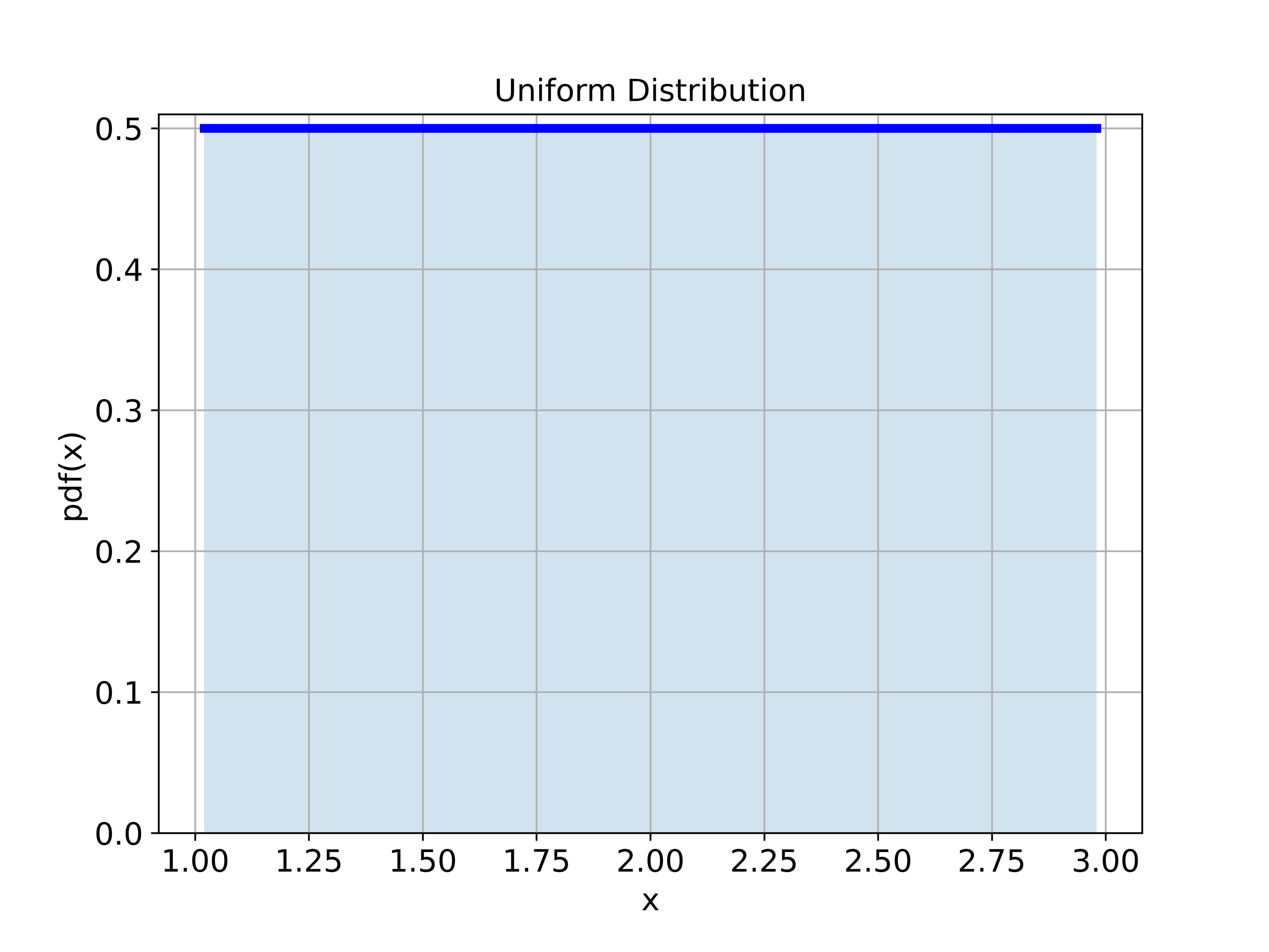
(11) $\begin{align*}\hat{I} & =\frac{(b-a)}{N}\sum_{i=1}^{N} g(x_{i})\end{align*}$

where $x_{i}$ samples are drawn from the uniform distribution on the interval $[a,b]$ . Let us verify this by using this function

(12) $\begin{align*}g(x)=x^{3}\end{align*}$

and the interval $[1,3]$ . The integral is

(13) $\begin{align*}\hat{I} = \int_{a=1}^{b=3} x^{3}\text{d}x=\frac{x^{4}}{4}\Bigg|_{a=1}^{b=3}=\frac{1}{4}\Big(3^{4}-1^{4} \Big)=\frac{80}{4}=20\end{align*}$

The Python script given below creates a uniform distribution and approximates the integral

import numpy as np
from scipy import stats
import matplotlib.pyplot as plt

# define a uniform distribution in Python on the interval [a,b+1]
a=1
b=2

# create a uniform distribution 
distribution=stats.uniform(a, b)

# plot the probability density function of the distribution
# start point
startPointXaxis=distribution.ppf(0.01)
# end point
endPointXaxis=distribution.ppf(0.99)

# create the x values
xValue = np.linspace(startPointXaxis,endPointXaxis, 500)

# the function pdf() will return the probability density function values
yValue = distribution.pdf(xValue)


# plot the probability density function
plt.figure(figsize=(8,6))
plt.gca()  
plt.plot(xValue,yValue, color='blue',linewidth=4)
plt.fill_between(xValue, yValue, alpha=0.2)
plt.title('Uniform Distribution', fontsize=14)
plt.xlabel('x', fontsize=14)
plt.ylabel('pdf(x)',fontsize=14)
plt.tick_params(axis='both',which='major',labelsize=14)
plt.grid(visible=True)
plt.xlim((startPointXaxis-0.1,endPointXaxis+0.1)) 
plt.ylim((0,max(yValue)+0.01)) 
plt.savefig('uniformDistribution2.png',dpi=600)
plt.show()



# generate random samples from the normal distribution
# and compute the variance estimate
sampleSize1=10
randomSamples1 = distribution.rvs(size=sampleSize1)
sum1=[(x)**3 for x in randomSamples1]
integralEstimate1=(b-a+1)*np.array(sum1).mean()



sampleSize2=20
randomSamples2 = distribution.rvs(size=sampleSize2)
sum2=[(x)**3 for x in randomSamples2]
integralEstimate2=(b-a+1)*np.array(sum2).mean()


sampleSize3=40
randomSamples3 = distribution.rvs(size=sampleSize3)
sum3=[(x)**3 for x in randomSamples3]
integralEstimate3=(b-a+1)*np.array(sum3).mean()


sampleSize4=100
randomSamples4 = distribution.rvs(size=sampleSize4)
sum4=[(x)**3 for x in randomSamples4]
integralEstimate4=(b-a+1)*np.array(sum4).mean()

The uniform distribution is given in the figure below.

The approximation results are given below

integralEstimate1=15.01969583856625
integralEstimate2=23.308232850684064
integralEstimate3=18.154486022709897
integralEstimate4=22.051801180232648

Basic Idea of the Monte Carlo Method – Intro Example

Basic Idea of the Monte Carlo Method – Integral of Nonlinear Function of Random Variable

Basic Idea of the Monte Carlo Method – Approximation of Deterministic Integrals

admin

You might also like

Clear and Concise Particle Filter Tutorial with Python Implementation- Part 1: Problem Formulation

How to Save Graphs to Image or PDF Files in Python by Using Pyplot and Matplotlib

State-Space Modeling of Double Mass-Spring-Damper System with Python Modeling