How to Detect and Draw Contours of Objects in OpenCV

In this OpenCV and Python tutorial, we explain how to detect object contours and how to draw them on the display screen. This is one of the fundamental operations that you will perform in many computer vision and object detection algorithms. Consequently, it is very important to know how to perform this operation in OpenCV and Python. The YouTube video accompanying this webpage is given below.

First, we demonstrate how to detect object contours by using an example of a rectangle. The image is shown below.

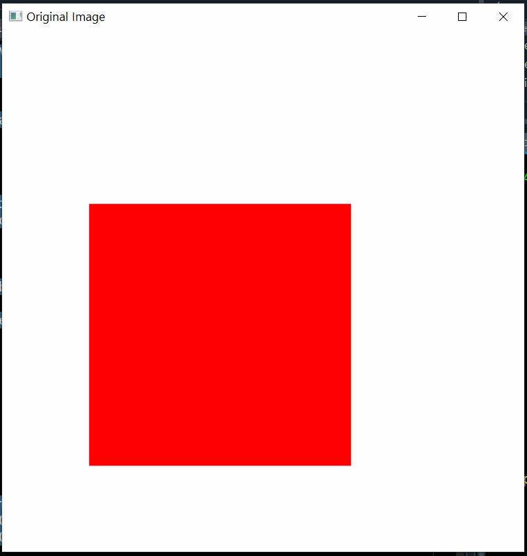
In our previous tutorial, whose link is given here, we explained how to draw rectangles in OpenCV. In this tutorial, we use the same approach to construct a rectangle. The Python script given below creates an image with a white background, draws a rectangle, and saves the image.

# import the necessary libraries
import numpy as np
import cv2
 
 
# create an image with a white background that serves as a drawing canvas
# set the width and height of the image
heightImage=600
widthImage=600
 
# a new image with a white background
# BGR (255,255,255)
newImageWhite = np.zeros((heightImage,widthImage,3),np.uint8)
# blue channel 
newImageWhite[:,:,0]=255
# green channel
newImageWhite[:,:,1]=255
# red channel
newImageWhite[:,:,2]=255
 

# draw a rectangle
# (x coordinate, y coordinate)
topLeftCornerPoint =(100,200)
bottomRightCornerPoint =(400,500)
 
# Rectangle color
colorRectangle=(0,0,255)
 
# create the rectangle 
cv2.rectangle(newImageWhite,topLeftCornerPoint,
             bottomRightCornerPoint,
             colorRectangle,-1)
 
# show the image with the rectangle
cv2.imshow("Original Image",newImageWhite)
cv2.waitKey(0)
cv2.destroyAllWindows()
 
 
# save image
cv2.imwrite("rectangleImageOriginal.png", 
            newImageWhite, [cv2.IMWRITE_PNG_COMPRESSION, 0]) 

To detect object contours in OpenCV, we need to perform the following three steps:

1. Convert color image to grayscale. In OpenCV, images are represented in the BGR color format (B- blue, G-green, and R-red). That is, every image is a NumPy array with the following dimensions: (width, height, 3), where the number 3 represents the three BGR color channels. On the other hand, grayscale images are represented by NumPy arrays with the following dimensions (width, height). The value stored at every entry represents a shade of gray.
2. Perform image thresholding. That is, apply the threshold operation to the image pixels. This operation converts a grayscale image to a binary image whose pixels can have two values. The values are zero and some other maximum value set by the user (usually 255). The thresholding operation sets the pixel value to zero if its value in the grayscale image is smaller than a threshold parameter. Otherwise, the pixel value is set to the maximum value. The threshold parameter is set by the user.
3. Determine the image contours by using the binary image as an input.

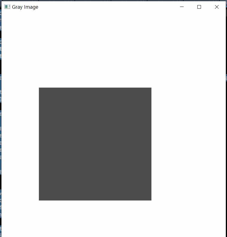
STEP 1: Convert Color Image to Grayscale. The Python script given below converts the color image to a grayscale image and shows the image on the screen.

# convert the image to grayscale 
grayImage = cv2.cvtColor(newImageWhite, cv2.COLOR_BGR2GRAY)


# show the grayscale image 
cv2.imshow("Gray Image",grayImage)
cv2.waitKey(0)
cv2.destroyAllWindows()

The image is shown below.

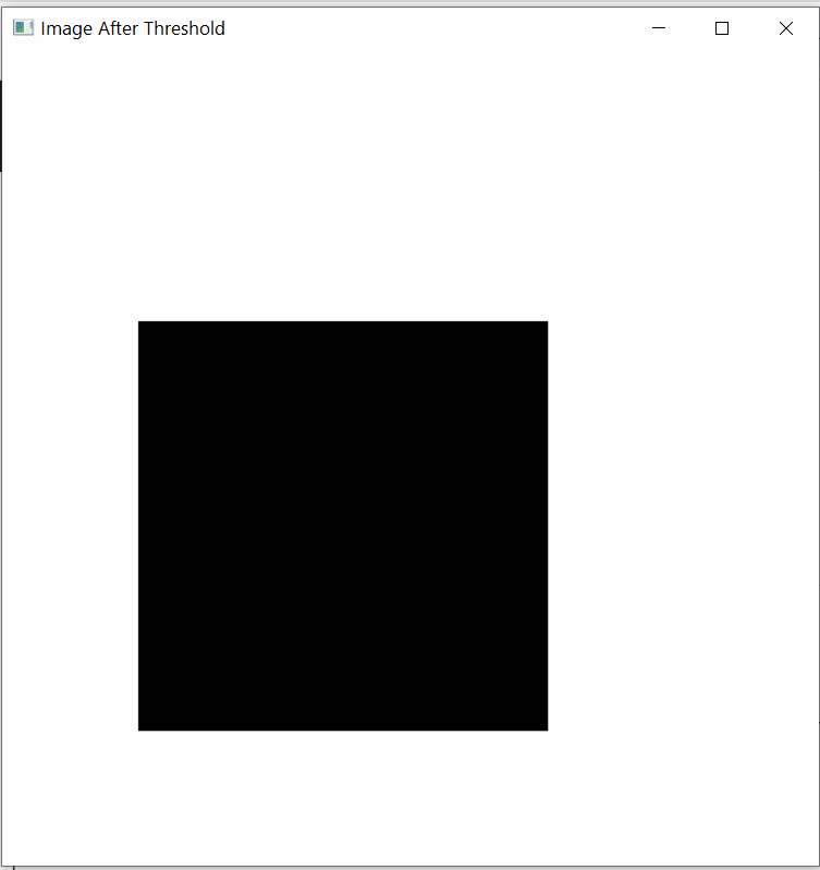
STEP 2: Perform Image Thresholding. To threshold the grayscale image, we use the OpenCV function “cv2.threshold()”. The first input argument of this function is a grayscale image. The second input argument is the threshold parameter. If the pixel value in the grayscale image is smaller than this parameter, the pixel value is set to zero, otherwise, it is set to a maximum value. The maximum value is the third input argument of the function. The final input argument is the flag indicating the type of thresholding. In our case, we use “cv2.THRESH_BINARY”. This is a simple binary thresholding. The Python script given below is used for thresholding.

# find the minimum and maximum values
# minimum value - this is the color of the rectangle after
# converting the image to gray image 
grayImage.min()
# maximum value - this is the white background color
grayImage.max()

# apply the threshold operation on the image 
# the first input argument to cv2.threshold should be a grayscale image 

# the second input argument is the threshold value 
# if the pixel value is smaller than the threshold value
# the value of the pixel is assigned to zero

# the third input argument is the value that is assigned to 
# the pixel values if they exceed the threshold value

# the function returns the computed threshold value thresValue
# and the image after the threshold operation threshImage
thresValue, threshImage = cv2.threshold(grayImage, grayImage.min()+1, 255, 
                                        cv2.THRESH_BINARY)

threshImage.min()
threshImage.max()


cv2.imshow("Image After Threshold",threshImage)
cv2.waitKey(0)
cv2.destroyAllWindows()

The binary image is shown below.

STEP 3: Determine the image contours: To determine the image contours, we use the OpenCV function “cv2.findContours(). The Python script given below extracts the contours and draws the specified contour on the screen.

# find contours 

contours, hierarchy = cv2.findContours(threshImage, 
                                           cv2.RETR_TREE, 
                                           cv2.CHAIN_APPROX_SIMPLE)

cv2.drawContours(newImageWhite, contours, 1, (0,255,0), 6)
cv2.imshow('Output Image', newImageWhite)
cv2.waitKey(0)
cv2.destroyAllWindows()

The first input argument of the function is the binary image. The second input argument “cv2.RETR_TREE” is a flag for the contour retrieval mode. This flag means that we are extracting all the contours and reconstructing the full hierarchy of the contours. The hierarchy of contours is organized as a tree data structure. The third argument “cv2.CHAIN_APPROX_SIMPLE” is a flag for the contour approximation method. “cv2.CHAIN_APPROX_SIMPLE” is a flag for the method that compresses horizontal, diagonal, and vertical segments. The segments are only represented by their end points. The first output of this function, denoted by “contours” in our code, is a tuple whose entries are contours. Every entry of this tuple is an array representing points of the contour. For example, in our case, “contours” has the following form

(array([[[  0,   0]],
 
        [[  0, 599]],
 
        [[599, 599]],
 
        [[599,   0]]], dtype=int32),
 array([[[ 99, 200]],
 
        [[100, 199]],
 
        [[400, 199]],
 
        [[401, 200]],
 
        [[401, 500]],
 
        [[400, 501]],
 
        [[100, 501]],
 
        [[ 99, 500]]], dtype=int32))

Besides the contour of the rectangle, the contour detection algorithm also determines the contour of the image. The second output of the function “cv2.findContours()” is the array encoding the hierarchy of the extracted contours. For a complete description of the contour hierarchy, see this explanation. The row numbers of the array “hierarchy” correspond to the index of the detected contours. The entries of every row of the hierarchy array are:

[Next Contour, Previous Contour, First Child, Parent Contour]

The contours are organized in a hierarchical way. “Next Contour” is the contour that is next to the current contour in the same hierarchical level. “Previous Contour” is the contour that is previous to the current contour in the same hierarchical level. “First Child” is the contour that is inside of the current contour. “Parent Contour” is the contour that is enclosing the current contour. If any of these objects do not exist, then the number is -1. In our case, the array “hierarchy” is

array([[[-1, -1,  1, -1],
        [-1, -1, -1,  0]]], dtype=int32)

There are two contours, and consequently, we have two rows. Let us analyze the first row that corresponds to the outer contour of our image:

[-1, -1,  1, -1]

The number of this contour is “0” and this corresponds to the first row of “hierarchy”. The first “-1” means that there is no next contour at the same level. Similarly, the second “-1” means that there is no previous contour at the same hierarchical level. The third “1” means that the contour number “1” is a child of the contour “0”. The fourth “-1” means that there is no parent contour of the current contour. Let us analyze the second row:

[-1, -1, -1,  0]

The index of this contour is “1” (the second row of “hierarchy”). The first “-1” means that there is no next contour at the same level. Similarly, the second “-1” means that there is no previous contour at the same level. The third “-1” means that there is no child contour of this contour. Finally, the last “0” means that the parent contour is the contour with the index “0”. This is exactly the outer contour of the image.

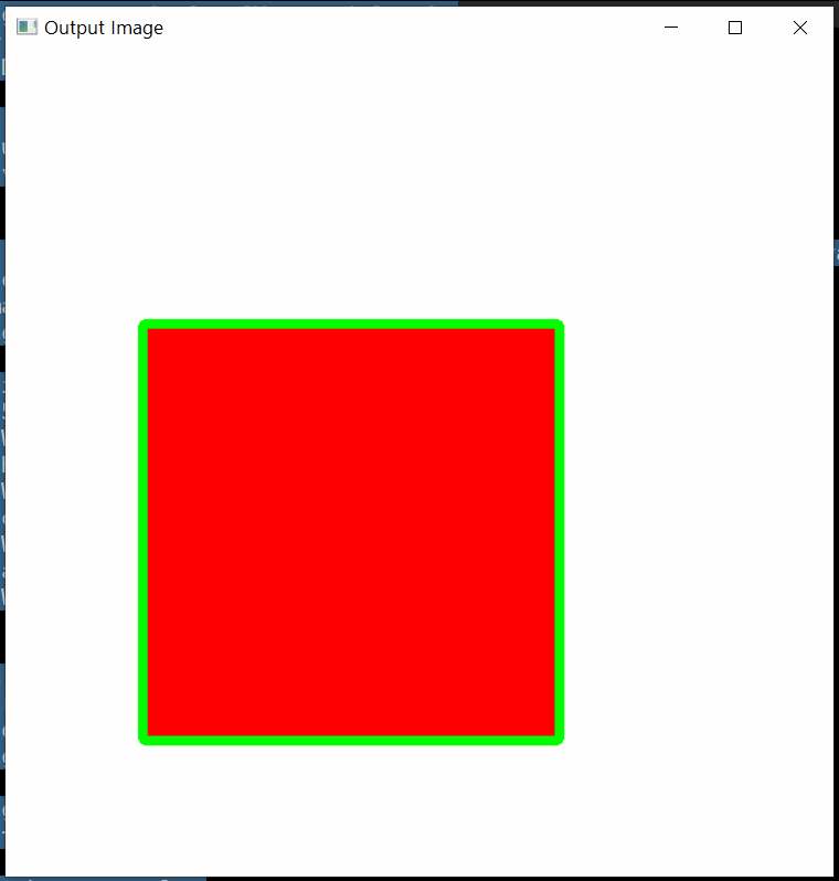
To draw the contours, we use the function “cv2.drawContours()”:

cv2.drawContours(newImageWhite, contours, 1, (0,255,0), 6)

The first input is the canvas image on which we want to draw the contours. The second input is the array of contours. The third input is the index of the contour that we want to draw. If we want to draw all the contours, then this index is set to -1. The fourth input is the BGR color code of the contour. The fifth index is the line thickness of the contour. The generated image with the green contour is given below.