Pole Placement With Integral Control Action to Eliminate Steady-State Error (State-Space Control Design) – Fusion of Engineering, Control, Coding, Machine Learning, and Science

In this post, we explain how to integrate an integral control action into a pole placement control design in order to eliminate a steady-state error. The YouTube video accompanying this post is given below

First, we explain the main motivation for creating this tutorial. When designing control algorithms, we are primarily concerned with two design challenges. First of all, we have to make sure that our control algorithm behaves well during the transient response. That is, as designers we specify the acceptable behavior of the closed-loop system during the transient response. For example, we want to make sure that the rise time (settling time) is within a certain time interval specified by the user. Also, we want to ensure that the system’s overshoot is below a certain value. For example, below 10 or 15 percent of the steady-state value. Secondly, we want to make sure that the control algorithm is able to eliminate the steady-state control error.

In your introductory course on control systems, you have probably heard of a pole placement problem and the solutions. The classical pole placement method is used to stabilize the system or for improving the transient response. This method finds a state feedback control matrix that assigns the poles of the closed-loop system to desired locations specified by the user. However, it is not obvious how to use the pole placement method for set-point tracking and for eliminating steady-state error in set-point tracking design problems. This tutorial explains how to combine the pole placement method with an integral control action in order to eliminate steady-state error and achieve a desired transient response. The technique presented in this lecture is very important for designing control algorithms.

Consider the following state-space model:

(1) $\begin{align*}\dot{\mathbf{x}} & =A\mathbf{x}+Bu \\y&=C\mathbf{x}\end{align*}$

where $\mathbf{x}\in \mathbb{R}^{n}$ , $u \in \mathbb{R}$ , and $y\in \mathbb{R}$ are state vector, input, and output. Here for presentation simplicity, we consider a single-input single-output system.

The classical pole placement design finds the feedback control matrix $K$ and the control law $u=-K\mathbf{x}$ such that the closed-loop system

(2) $\begin{align*}\dot{\mathbf{x}} & =\big(A-BK\big) \mathbf{x}\end{align*}$

is stable and that the poles are placed at the desired locations (that are specified by the designer). The issue with this approach is that although we can place the poles at the desired locations, we do not have full control of steady-state error.

The basic idea for tackling this problem is to augment the original system (2) with an integrator of the error:

(3) $\begin{align*}x_{i}=\int \big(r-C\mathbf{x} \big) \text{dt}\end{align*}$

where $r$ is the set point (desired value of the output). By taking the first derivative of (3), we obtain

(4) $\begin{align*}\dot{x}_{i}=r-C\mathbf{x}\end{align*}$

where $x_{i}$ is an additional state. By combining the state-space model (2) and (4), we obtain

(5) $\begin{align*}\dot{\mathbf{x}} & =A\mathbf{x}+Bu \\\dot{x}_{i}&=r-C\mathbf{x} \\y&=C\mathbf{x}\end{align*}$

We can write (5) compactly

(6) $\begin{align*}\begin{bmatrix}\dot{\mathbf{x}} \\ \dot{x}_{i} \end{bmatrix} &=\begin{bmatrix}A & 0 \\ -C & 0 \end{bmatrix}\begin{bmatrix} \mathbf{x} \\ x_{i} \end{bmatrix}+\begin{bmatrix} B \\ 0 \end{bmatrix}u+\begin{bmatrix} 0 \\ 1 \end{bmatrix}r \\y&=\begin{bmatrix}C & 0 \end{bmatrix}\begin{bmatrix} \mathbf{x} \\ x_{i} \end{bmatrix}\end{align*}$

From the last system of equations, we can observe that we have formed a new state-space model, with the state variable:

(7) $\begin{align*}\begin{bmatrix} \mathbf{x} \\ x_{i} \end{bmatrix}\end{align*}$

The state-feedback controller now has the following form

(8) $\begin{align*}u=- \underbrace{\begin{bmatrix} K_{x} & K_{i} \end{bmatrix}}_{K}\begin{bmatrix} \mathbf{x} \\ x_{i} \end{bmatrix} =-K_{x} \mathbf{x} - K_{i}x_{i}\end{align*}$

where $K$ is the state feedback control matrix consisting of the original state feedback control matrix $K_{x}$ and integral control feedback matrix $K_{i}$ . Note here that is, the states of the original system (1) are the position $p$ and velocity $\dot{p}$ , and if the position is measured, then the control law (8) have some similarities with a PID controller. We can design the matrix $K$ and its block matrices by using the MATLAB function place().

By substituting the feedback control algorithm (8) in the state-space model (6), we obtain the following system

(9) $\begin{align*}\begin{bmatrix}\dot{\mathbf{x}} \\ \dot{x}_{i} \end{bmatrix} &=\begin{bmatrix} A & 0 \\ -C & 0 \end{bmatrix}\begin{bmatrix} \mathbf{x} \\ x_{i} \end{bmatrix}-\begin{bmatrix}B \\ 0 \end{bmatrix}\begin{bmatrix} K_{x} & K_{i} \end{bmatrix}\begin{bmatrix} \mathbf{x} \\ x_{i} \end{bmatrix}+\begin{bmatrix} 0 \\ 1 \end{bmatrix}r \\ \begin{bmatrix}\dot{\mathbf{x}} \\ \dot{x}_{i} \end{bmatrix} &=\begin{bmatrix} A & 0 \\ -C & 0 \end{bmatrix}\begin{bmatrix} \mathbf{x} \\ x_{i} \end{bmatrix}-\begin{bmatrix} BK_{x} & BK_{i} \\0 & 0 \end{bmatrix}\begin{bmatrix} \mathbf{x} \\ x_{i} \end{bmatrix}+\begin{bmatrix} 0 \\ 1 \end{bmatrix}r \\\begin{bmatrix}\dot{\mathbf{x}} \\ \dot{x}_{i} \end{bmatrix} &=\begin{bmatrix} A-BK_{x} & -BK_{i} \\ -C & 0 \end{bmatrix}\begin{bmatrix} \mathbf{x} \\ x_{i} \end{bmatrix}+\begin{bmatrix} 0 \\ 1 \end{bmatrix}r \end{align*}$

The new system matrix

(10) $\begin{align*}A_{\text{new}}=\begin{bmatrix} A-BK_{x} & -BK_{i} \\ -C & 0 \end{bmatrix}\end{align*}$

Is the Hurwitz matrix (all its eigenvalues have strictly negative real parts). Consequently, transient response due to non-zero initial conditions will die out after some time, and the output of the system will asymptotically approach the reference value, given by $r$ .

Next, we present MATLAB codes for implementing this control approach. The following code lines define the system, compute eigenvalues of the open-loop system, perform basic diagnostics, and compute the open-loop response.

clear,pack,clc
% define the system matrices
A=[0 1; -2 -4];
B=[0; 1];
C=[1 0]
D=[]
% open loop poles 
polesOpenLoop=eig(A)

% define the state-space model
systemOpenLoop=ss(A,B,C,D)

% check the step response in order to check the steady-state error
step(systemOpenLoop)

The open-loop step response is given below.

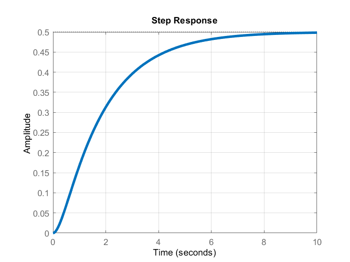
Figure 1: Open-loop step response of the defined system.

The open-loop system is asymptotically stable. However, we can observe that we have a significant steady-state error. To eliminate the steady-state error, we use the developed approach.

Next, we define the augmented system for pole placement, define desired closed-loop poles, compute the feedback control gain, define the close-loop system, compute the transfer function of the system, and compute the step response. The following code lines are used to perform these tasks.

% define the augmented system for pole placement
At=[A zeros(2,1);
    -C 0];
Bt=[B;0];
Br=[zeros(2,1);1];

% define the desired close-loop system poles
% here the logic is to push the open-loop poles for the distance of 3 times
% the original distance from the imaginary axis, and to push an additional
% pole due to the integral action further left - 10 times the distance of
% the minimal open-loop pole

desiredClosedLoopPoles=[3*polesOpenLoop;
                        10*min(polesOpenLoop)];

% compute the feedback control gain K
K=place(At,Bt,desiredClosedLoopPoles)

% define the close-loop system for simulation
Acl=At-Bt*K
% check the eigenvalues in order to ensure that they are properly assigned
placedPoles=eig(Acl)

% check the error in placing the poles
sort(desiredClosedLoopPoles)-sort(placedPoles)

% close-loop C matrix
Ccl=[C 0]
Dcl=[]

% here we define the close-loop system
systemCloseLoop=ss(Acl,Br,Ccl,Dcl)

% compute the transfer function of the system
tf(systemCloseLoop)

% compute the step response from the reference input
step(systemCloseLoop)

The resulting step response of the system is shown in the figure below.

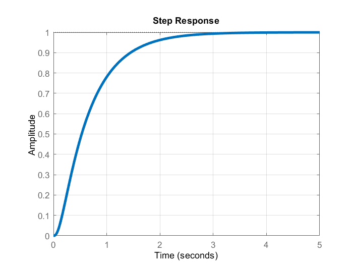
Figure 2: Closed-loop system response after adding an integral action and performing pole placement.

A few comments about the presented code are in order. In code line 13, we define the closed-loop poles. We shift the open-loop poles to left compared to their original location in order to ensure a faster response. Also, we set an additional pole corresponding to the introduced integral action to be a shifted version of the open-loop pole with the minimal real part (maximal absolute distance from the imaginary axis). From the step response of the closed-loop system, we can observe that the steady-state error has been eliminated. Consequently, our control system with the additional integral action is able to successfully track reference set points. The computer transfer function of the closed-loop system is

(11) $\begin{align*}W(s)=\frac{614.6}{s^3 + 46.14 s^2 + 427.7 s + 614.6}\end{align*}$

From this transfer function, we can observe that the gain of the system is $1$ . Consequently, we the system is able to track constant reference signals.

That would be all. A related post to this post and tutorial is a tutorial on how to compute a Linear Quadratic Regulator (LQR) optimal controller. That tutorial can be found here.

admin

You might also like

Design and Test Observers of Dynamical Systems in MATLAB

Implementation of the Solution of the Linear Quadratic Regulator (LQR) Control Algorithm in C++ by Using the Eigen Matrix Library.

Z-Transform Introductory Tutorial with Examples of Z-Transform of Unit Impulse Sequence and Unit Step Sequence