 by
by
In this control engineering and control theory tutorial, you will learn how to design and test observers of dynamical systems in MATLAB. We focus on linear dynamical systems in the state-space form. We explain how to design observers by using the pole placement method, and how to numerically implement and test the performance of observers in MATLAB.
This webpage tutorial is organized as follows. First, we briefly explain the basics of observers for linear dynamical systems in state-space form. Then, we explain how to design observer gain matrices by using the pole placement method. Finally, we explain how to implement observers in MATLAB and how to numerically test their performance. Before reading this tutorial, we strongly suggest that the interested reader thoroughly studies our previous tutorial, given here, which explains the basics of state observers. That tutorial also explains how to implement the obsevers in Python. However, the Python implementation is not important since in this webpage tutorial we explain how to implement observers in MATLAB.
The YouTube tutorial accompanying this webpage tutorial is given below.
Basics of Observers of Linear Dynamical Systems in the State Space Form
We consider the following linear state-space model of a dynamical system:
(1) 
where  is the state vector,
  is the control input vector,
  is the output vector, and
  and
and  are the system matrices.
Here, it should be emphasized that ONLY the output vector  of the system (1) can be observed. However, in many applications, we would like to have access to the full state vector
  . For example, in order to design a state feedback control algorithm, we need to have information about the state vector . There are also many other scenarios in which we need information about the full-state vector. This motivates us to develop an algorithm that will estimate the state vector from the time sequence of the observed output vector . Such an algorithm is called an observer in the control engineering literature.
Consequently:
The main goal of an observer is to estimate the state of the system (1) from the measurements of the output vector.
Also, it should be emphasized that when designing the observer, we assume that the system matrices  and
and  of the state-space model (1) are known. Under this assumption, the observer of the system (1) is given by the following state equation
(2) 
here  is the state of the observer, and
  is the observer gain matrix. Here, several important things need to be kept in mind
- The “hat” notation denotes the state of the observer that is at the same time an estimate of the state . That is, the state of the observer is the estimate of the system state vector .
- The matrix is the observer gain matrix. Our goal is to design this matrix such that the state of the observer asymptotically tracks the state of the system . Equivalently, we want to design the observer gain matrix such that the state estimation error
 asymptotically approaches zero. As we explain later on, this means that the closed-loop dynamics of the observer has to be stable.
 - By discretizing the observer (2) state equation we can obtain a recursive difference state equation which can be implemented in a microcontroller or FPGA. That is, the observer is actually an algorithm that can be implemented in a digital computer. Also, it should be kept in mind that at any time instant, we know the state of the observer. However, we do not know the exact value of the state of the system.
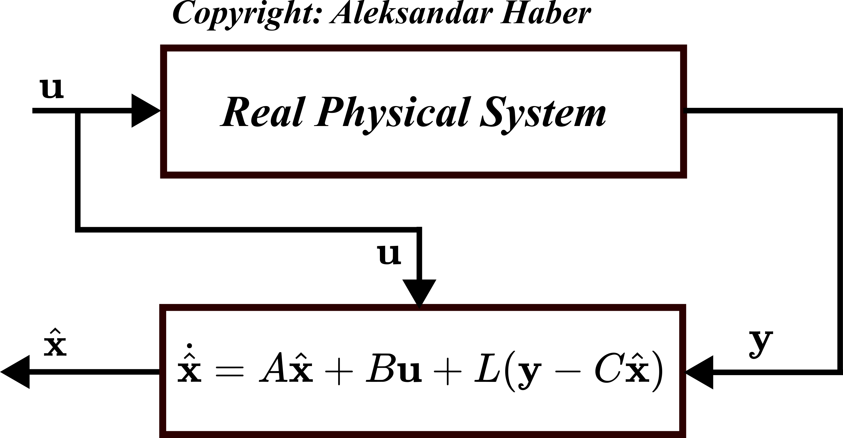
The block diagram of the observer is shown below.
Design and Simulation of State Observer in MATLAB
Here, we explain how to use the pole placement method to design state observers in MATLAB. That is, our goal is to compute the matrix of the state observer (2). First, let us define the estimation error
(3) 
Let us take the first derivative of this equation. As a result, we obtain
(4) 
By substituting state equations of the dynamical system (1) and observer (2) in (4), we obtain
(5) 
From the last equation, we obtain
(6) 
where we used the fact that  . By using the equation (3), from (6) we obtain
(7) 
The equation (7) represents the closed-loop observer dynamics. The goal of the observer design is to select the matrix such that the closed loop system (7) is asymptotically stable.
The closed-loop stability of the system is achieved by using the pole placement method. The idea is to design the matrix such that the eigenvalues of the matrix  are at prescribed locations.
MATLAB has a function called “place()” to perform pole placement. However, this function is designed for feedback control problems where the goal is to compute the feedback control matrix  such that the poles of the closed-loop system
(8) 
are at prescribed locations. However, our observer design problem looks a bit different. Our closed-loop matrix is
(9) 
That is, the positions of and matrices are different. However, we can still use the place function by observing the following. First of all, it is a very well-known fact that a matrix and its transpose have the same eigenvalues. This means that the matrix (9) and its transpose matrix
(10) 
have the same set of eigenvalues. We can observe that the matrix (10) has the same structure as the matrix (8), where  plays the role of
  ,
,  plays the role of
  , and
, and  plays the role of .
As a test case, we consider the system shown in the figure below.
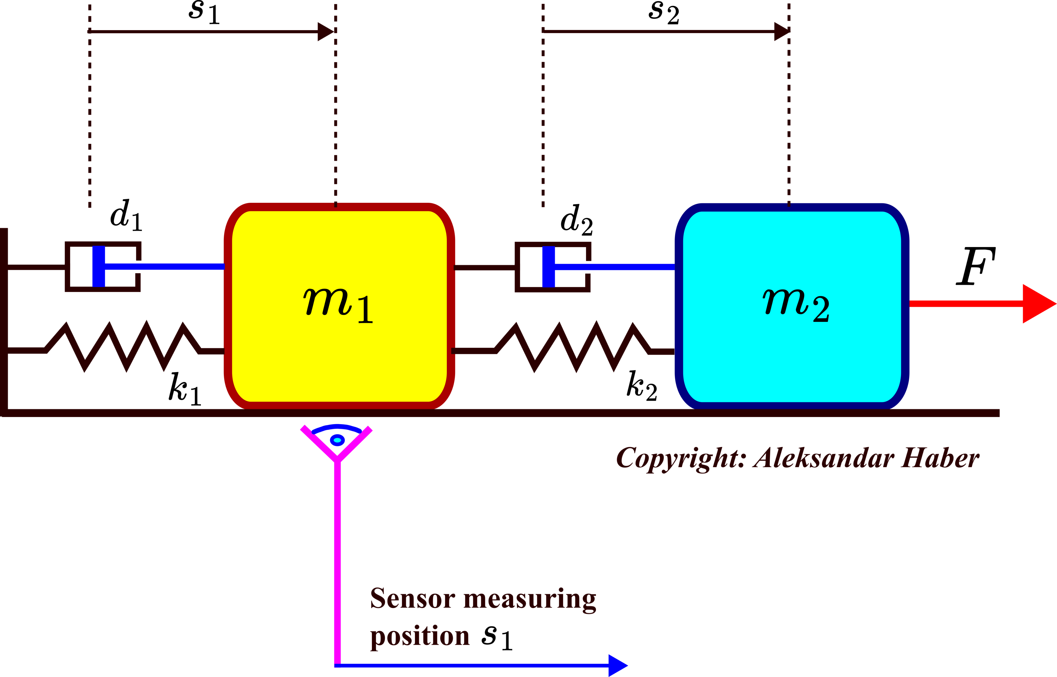
The system consists of two objects with masses of  and
and  that are connected by two springs and dampers. The spring constants are
  and
and  , and the damping constants are
  and
and  . The external force
  is used to control the system. The variables
  and
and  are displacements of the objects from their equilibrium positions. We assume that only the displacement can be observed.
In our previous tutorial, which can be found here, we derived a state-space model of this system. The state-space model is derived by assigning the following state-space variables
(11) 
where  and
and  are the velocities of the first and second object. The state-space model has the following form
(12) 
where
(13) 
Our first task is to model and simulate the mass-spring-damper system in MATLAB. The following MATLAB script is used to achieve this
clear
% system parameters
m1=5; m2=10;
k1=10; k2=20;
d1=5; d2=10;
% state space matrices
A=[0 1 0 0;
-(k1+k2)/m1 -(d1+d2)/m1 k2/m1 d2/m1;
0 0 0 1;
k2/m2 d2/m2 -k2/m2 -d2/m2]
B=[0; 0; 0; 1/(m2)]
C=[1 0 0 0]
D=[]
% simulate the system to obtain the state-space response
sys1=ss(A,B,C,D)
timeVector=0:0.1:5
input=10*ones(size(timeVector))
X0true=[3;1;-3;-2]
[yTrue,timeTrue,xTrue] = lsim(sys1,input,timeVector,X0true)
figure(1)
hold on
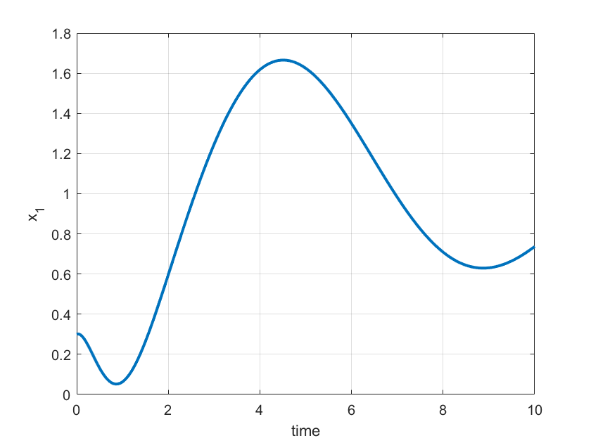
plot(timeTrue,xTrue(:,1))First, we define the system parameters and system matrices. Then, we use MATLAB’s function “ss()” to define the state-space model of the system. Then, we define the simulation parameters. We define the time vector and the input vector. The input vector is the time series of force values applied to the second object. In our case, we assume a constant input. Then, we simulate the system by using the function “lsim()”. The first input argument of lsim() is the system’s state-space model. The second input argument is the input vector that is applied to the system. The third input argument is the time vector for simulation. The final input argument is the initial state for simulation. The function lsim() returns the simulated output sequence, time vector, and simulated state sequence. Finally, we plot the simulation result. The figure below shows the time sequence of the state  .
.
 .
.Next, we design the observer gain matrix . The MATLAB script is given below.
% desired pole locations
poleLocation=[-4; -6; -2+2i; -2-2i]
% determine the transpose of the observer gain matrix
Lt = place(A',C',poleLocation)
% observer gain matrix
L=Lt'
% compute the closed-loop matrix
Acl=A-L*C
% check the closed-loop eigenvalues
polePlaced=eig(Acl)

% check the location is correct
abs(sort(poleLocation)-sort(polePlaced))
First, we specify a vector of desired pole locations. The vector name is “poleLocation”. We want to place the poles of the closed-loop matrix at the following locations:
(14) 
Then, we use the function place() to design the matrix . As explained previously, we pass to this function the transposes of and , and as the final argument, we pass the vector of desired pole locations “poleLocation”. The function place() returns the transpose of the matrix . Consequently, in the following code line, we transpose the matrix . We then compute the closed-loop observer matrix and we check the eigenvalues of the matrix. The eigenvalues of the closed-loop matrix are computed pole locations. Finally, we double-check that the computed pole locations are correct by comparing the vectors of desired pole locations and the computed pole locations. Next, we simulate the designed observer. To simulate the design observer, we need to transform the state-space model of the observer in the appropriate form. The observer is given by the equation (2). This equation can be written as follows
(15) 
The last equation can be written as
(16) 
Next, we need to assign an output equation to our observer. We select the output matrix of the observer as an identity matrix. We can do that since we know the observer’s state. Consequently, the output equation of the observer has the following form
(17) 
where  is the output of the observer, and the observer matrix
  is an identity matrix defined by
(18) 
The complete state-space model of the observer takes the following form
(19) 
where
(20) 
In the observer state-space model (19) the vector  consisting of the input
  and the output of the system is the input of the observer (see Fig. 1 at the top of this video tutorial for the block diagram of the observer).
The script given below creates a state-space model and simulates the observer.
% simulate the closed loop observer
% we need to create another state-space model representing the observer
Aobserver=Acl
Bobserver=[B L]
Cobserver=eye(4,4)
Dobserver=[]

% create the observer state-space model
sysObserver=ss(Aobserver,Bobserver,Cobserver,Dobserver)

% create a new augmented input sequence matrix
% consisting of the inputs and outputs of the original system
inputUY=[input;yTrue';]

% this is the initial state of the observer that is at the same time
% an initial guess of the system state
X0observer=[0;0;0;0];

% here, we simulate he observer
[yObserver,timeObserver,xObserver] = lsim(sysObserver,inputUY,timeVector,X0observer);

% here, we plot the observer state and the true state of the system
figure(2)
hold on
plot(timeTrue,xTrue(:,2),'r')
plot(timeObserver,xObserver(:,2),'b')
First, we create the observer state-space matrices and create the observer state-space model by using the function ss(). Next, by using the following code line
inputUY=[input;yTrue';]we create the observer input time sequence. The observer input consists of the input and output sequences of the original system. After defining this input sequence, we select an initial state of the observer, denoted by “X0observer”. This initial state is at the same time the initial guess of the system’s state. Then, we simulate the observer behavior by using the function “lsim()”. Finally, we plot the observer and system state. The results are shown in the figures below.
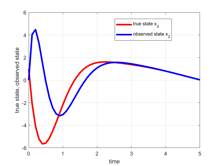
 and the observer state
  .
.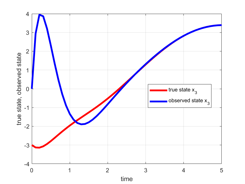
 and the observer state
  .
.From the two figures shown above, we can observe that the observer’s initial state quickly converges to the true state of the system. This means that the observer is properly designed.