Convert State-Space Models into Transfer Functions with MATLAB Codes – Fusion of Engineering, Control, Coding, Machine Learning, and Science

In this post, and in the accompanying video tutorial, we explain how to convert state-space models into transfer functions. We explain how to perform this conversion analytically and in MATLAB. The YouTube video tutorial accompanying this post is given below.

Consider the following state-space model

(1) $\begin{align*}\dot{\mathbf{x}}=A\mathbf{x}+B\mathbf{u} \\\mathbf{y}=C\mathbf{x}+D\mathbf{u}\end{align*}$

where $\mathbf{x}\in \mathbb{R}^{n}$ is the state vector, $\mathbf{u}\in \mathbb{R}^{m}$ is the input vector, and $\mathbf{y}\in \mathbb{R}^{r}$ is the input vector, the matrices $A\in \mathbb{R}^{n\times n},B\in \mathbb{R}^{n\times m}$ , $C\in \mathbb{R}^{r\times n}$ , and $D\in \mathbb{R}^{r\times m}$ are the system matrices.

Our goal is to convert this state-space model to a transfer function (also called a transfer matrix, since the system has multiple inputs and outputs): the transfer function will have the following form

(2) $\begin{align*}Y(s)=W(s)U(s)\end{align*}$

where $W(s)\in \mathbb{C}^{r \times m}$ is the transfer function and $s\in \mathbb{C}$ is the complex variable (obtained by applying the Laplace transform), and $Y(s)\in \mathbb{C}^{r}$ and $U(s)\in \mathbb{C}^{r}$ are the Laplace transforms of the output and input vectors. Note that the Laplace transforms of vector are denoted by capital letters.

Let us apply the Laplace transform to our original system (1). Since transfer functions are defined for zero initial conditions, we have to keep this fact in account while applying the Laplace transform. As the result, from (1), we obtain

(3) $\begin{align*}sX(s)=AX(s)+BU(s) \\Y(s)=CX(s)+DU(s)\end{align*}$

where $X(s)$ is the Laplace transform of the state vector. From the first equation, we have:

(4) $\begin{align*}\big(sI-A \big) X(s)=BU(s)\end{align*}$

where $I \in \mathbb{R}^{n\times n}$ is the identity matrix. From this equation, we have

(5) $\begin{align*}X(s)=\big(sI-A \big)^{-1}BU(s)\end{align*}$

where $\big(sI-A \big)^{-1}$ is an inverse of $\big(sI-A \big)$ . By substituting (5) in the output equation of (3), we obtain

(6) $\begin{align*}Y(s)=C\big(sI-A \big)^{-1}BU(s)+DU(s)=\Big(C\big(sI-A \big)^{-1}B+D\Big) U(s)\end{align*}$

The last equation can be written compactly

(7) $\begin{align*}Y(s)=W(s)U(s)\end{align*}$

where $W(s)$ is the transfer function

(8) $\begin{align*}W(s)=C\big(sI-A \big)^{-1}B+D \end{align*}$

In the case of single-input-single-output systems, the transfer function is not a matrix, and we can write

(9) $\begin{align*}\frac{Y(s)}{U(s)}=W(s)\end{align*}$

Problem: Find the transfer function of the following system

(10) $\begin{align*}\dot{\mathbf{x}} & =\begin{bmatrix} 0 & 1 & 0 \\ 0 & 0 &1 \\ -1 &-2 &-3 \end{bmatrix}\mathbf{x}+\begin{bmatrix} 10 \\ 0 \\ 0 \end{bmatrix}u \\y & =\begin{bmatrix}1 & 0 & 0 \end{bmatrix}\mathbf{x} \end{align*}$

Solution:

First, we compute $\big(sI-A\big)$ . We have

(11) $\begin{align*}sI-A= \begin{bmatrix} s & 0 & 0 \\ 0 & s & 0 \\ 0 & 0 & s \end{bmatrix}-\begin{bmatrix} 0 & 1 & 0 \\ 0 & 0 &1 \\ -1 &-2 &-3 \end{bmatrix}=\begin{bmatrix}s & -1 & 0 \\ 0 & s & -1\\ 1 & 2 & s+3 \end{bmatrix} \end{align*}$

The inverse matrix $\big(sI-A\big)^{-1}$ is defined by

(12) $\begin{align*}\big(sI-A\big)^{-1}=\frac{\text{adj}\big(sI-A\big)}{\text{det}\big(sI-A\big)}\end{align*}$

where $\text{adj}\big(sI-A\big)$ is the adjugate matrix of $\big(sI-A\big)$ and $\text{det}\big(sI-A\big)$ is the determinant matrix of $\big(sI-A\big)$ . The adjugate matrix is formed by transposing the cofactor matrix. The cofactor matrix of $\big(sI-A\big)$ is (see the video for the explanation on how to compute the cofactor matrix)

(13) $\begin{align*}C_{o}=\begin{bmatrix}s^{2}+3s+2 & -1 & -s \\ s+3 & s^2+3s &-2s-1 \\ 1 & s & s^2 \end{bmatrix}\end{align*}$

Consequently, the adjugate matrix is

(14) $\begin{align*}\text{adj}\big(sI-A\big)=C_{o}^{T}=\begin{bmatrix} s^2+3s+2 & s+3 & 1\\ -1 & s^2+3s & s\\ -s & -2s-1 &s^2 \end{bmatrix} \end{align*}$

The determinant of the matrix $\big(sI-A\big)$ is $\text{det}\big(sI-A\big)=s^3+3s^2+2s+1$

Finally, our transfer function matrix is:

(15) $\begin{align*}W(s)& =\frac{1}{s^3+3s^2+2s+1}\begin{bmatrix}1 & 0 & 0 \end{bmatrix}\begin{bmatrix} s^2+3s+2 & s+3 & 1\\ -1 & s^2+3s & s\\ -s & -2s-1 &s^2 \end{bmatrix} \begin{bmatrix} 10 \\ 0 \\ 0 \end{bmatrix} \\& =\frac{10\big(s^2+3s+2 \big)}{s^3+3s^2+2s+1} \end{align*}$

Below are the MATLAB codes for computing the transfer function. There are two approaches. Here is the first approach that relies upon the MATLAB Symbolic Toolbox.

% first approach for calculating the transfer function
syms s
A=[0 1 0;
    0 0 1;
    -1 -2 -3];
B=[10; 0; 0];
C=[1 0 0]
matrix1=s*eye(3)-A
matrix2=inv(matrix1)
transferFunction=C*matrix2*B

The command syms is used to define a symbolic complex variable $s$ . The other parts of the code are self-explanatory.

The second approach is given below. This approach relies upon the MATLAB Control System Toolbox.

% second approach for calculating the transfer function
clear, pack, clc
A=[0 1 0;
    0 0 1;
    -1 -2 -3];
B=[10; 0; 0];
C=[1 0 0];
D=[]

system1=ss(A,B,C,D)

transferFunction=tf(system1)

We define the state-space model by using the MATLAB function ss(). Then we transform such a state-space model into a transfer function form by using the command tf().

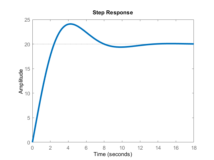
Below is the step response of the system computed by using the MATLAB function step().

admin

You might also like

Pole Placement Example 1- Design PID Controller to Achieve Desired Closed-Loop Behavior

Three Must-Know Methods For Computing Fibonacci Sequence in C++

Solve Constrained Optimization Problems in Python by Using SciPy Library, minimize() Function and Trust-Region Constrained Method