Pole Placement Example 1- Design PID Controller to Achieve Desired Closed-Loop Behavior – Fusion of Engineering, Control, Coding, Machine Learning, and Science

In this tutorial, we will solve one very important problem that every control or signal processing engineer needs to know how to solve. Namely, in this tutorial, we will learn how to use the pole placement method to select control algorithm parameters such that the poles of the closed-loop system are placed at the desired locations. More precisely, on the basis of the desired locations of the closed-loop poles, we will determine the parameters of the Proportional Integral Derivative or PID control algorithm. We will also see that the control algorithm will introduce zeros in the closed-loop transfer function that will slightly degrade the desired closed-loop response. The YouTube tutorial accompanying this control engineering tutorial is given below.

Problem Statement

We explain the procedure by using the example presented below.

PROBLEM STATEMENT: For a given open-loop transfer function

(1) $\begin{align*}W(s)=\frac{1}{s^{2}+4}\end{align*}$

Design a feedback controller such that the poles of the closed-loop transfer function are

(2) $\begin{align*}s_{1}=-2,\;\; s_{2}=-3,\;\; s_{3}=-4\end{align*}$

and such that the steady-state error of following a step reference signal is asymptotically equal to zero.

The YouTube tutorial explaining how to solve this problem is given below.

Solution

ANALYSIS AND COMMENTS: First, it should be observed that the open-loop transfer function has poles on the imaginary axis. This is not what we want. Such a system exhibits an oscillatory behavior and cannot accurately track a step reference signal. Consequently, we need a feedback control algorithm to asymptotically stabilize the system, and to make sure that the closed-loop system can asymptotically track a reference signal. Also, we want to place closed-loop poles on the real axis (this is the design task). We want to do that in order to ensure a smooth system response with minimal oscillations. That is, we will see the exponential terms

(3) $\begin{align*}\pm e^{-2t}, \;\; \pm e^{-3t},\;\; \pm e^{-4t}\end{align*}$

which will ensure a relatively damped response. However, we will also see that the controller will introduce zeros that will induce some oscillations and overshoot in the response.

SOLUTION: The block diagram of the closed-loop system is given below.

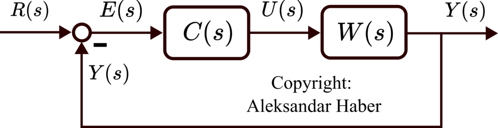
This block diagram is the system representation in the complex Laplace domain. Here $s$ is the complex Laplace variable. $C(s)$ is the controller that we want to determine. $R(s)$ is the reference signal that we want to follow, $U(s)$ is the output of the controller that is at the same time the input to the open loop transfer function $W(s)$ . $Y(s)$ is the output of the system. The control error is given by

(4) $\begin{align*}E(s)=R(s)-Y(s)\end{align*}$

The first step is to determine the closed-loop transfer function. We have

(5) $\begin{align*}Y(s)=W(s)U(s)=W(s)C(s)E(s)=W(s)C(s)\Big( R(s)-Y(s)\Big)\end{align*}$

From the last equation, we have

(6) $\begin{align*}\Big( 1+W(s)C(s)\Big) Y(s)=W(s)C(s)R(s)\end{align*}$

From the last equation, we obtain

(7) $\begin{align*} Y(s)=\frac{W(s)C(s)}{1+W(s)C(s) }R(s)\end{align*}$

From the last equation, we can see that the closed-loop transfer function is

(8) $\begin{align*}W_{cl}=\frac{W(s)C(s)}{1+W(s)C(s) }\end{align*}$

We are interested in the closed-loop poles of the system. The closed-loop poles are zeros of the characteristic polynomial of the closed-loop transfer function. The characteristic polynomial is determined by

(9) $\begin{align*}1+W(s)C(s)=0\end{align*}$

The open-loop transfer function is given by the equation (1), on the other hand, we have the freedom to choose the control transfer function. That is, we have the complete freedom to choose our control algorithm. Let us select the Proportional Integral Derivative (PID) control algorithm. The transfer function of the PID controller can be written in this form

(10) $\begin{align*}C(s)=\frac{K(as+1)(bs+1)}{s}\end{align*}$

where $K$ , $a$ , and $b$ are the controller parameters that we need to determine. To see that this is actually the PID controller, we can easily write the last transfer function as follows

(11) $\begin{align*}C(s)=\frac{K}{s}+K(a+b)+Kab\cdot s\end{align*}$

since $1/s$ is an integrator in the time domain, $s$ is a derivative action in the time domain, and a constant term in the Laplace domain is a proportional term in the time domain, in the time domain, the output of the controller is

(12) $\begin{align*}u(t)=K\int_{0}^{t} e(t) dt +K(a+b)e(t)+Kab\dot{e}(t)\end{align*}$

By substituting the controller (10) and the transfer function (1) into the equation for the characteristic polynomial (9), we obtain

(13) $\begin{align*}1+\frac{1}{s^{2}+4}\cdot \frac{K(as+1)(bs+1)}{s}=0\end{align*}$

By multiplying the last equation by $s(s^{2}+4)$ , we obtain

(14) $\begin{align*}s(s^{2}+4)+K(as+1)(bs+1)=0\end{align*}$

By multiplying the terms in the last equation and grouping them together, we obtain

(15) $\begin{align*}s^{3}+Kab\cdot s^{2}+(4+Ka+Kb)\cdot s+K=0\end{align*}$

On the other hand, our task is to assign the closed-loop poles at the following locations

(16) $\begin{align*}s_{1}=-2,\;\; s_{2}=-3,\;\; s_{3}=-4\end{align*}$

From this, we conclude that the desired characteristic polynomial of the closed-loop system should be

(17) $\begin{align*}(s+2)(s+3)(s+4)=0\end{align*}$

By multiplying the terms in the last expression, we obtain

(18) $\begin{align*}(s+2)(s+3)(s+4)=(s^{2}+5s+6)(s+4)=s^{3}+9s^{2}+26s+24=0\end{align*}$

By equating (15) and (18), we obtain

(19) $\begin{align*}s^{3}+Kab\cdot s^{2}+(4+Ka+Kb)\cdot s+K=s^{3}+9s^{2}+26s+24\end{align*}$

Two polynomials are equal if their coefficients are equal. By using this fact, and the last equation, we obtain

(20) $\begin{align*}K=24\\4+Ka+Kb=26 \\Kab=9 \end{align*}$

Since the first equation gives $K=24$ , by substituting this expression in the second and third equation, we obtain

(21) $\begin{align*}a+b=\frac{11}{12} \\ab=\frac{3}{8}\end{align*}$

By multiplying the first equation with $a$ , we obtain

(22) $\begin{align*}a^{2}+ab=\frac{11}{12}a \\\end{align*}$

Then, by substituting the second equation from (21) into (22), we obtain

(23) $\begin{align*}a^{2}-\frac{11}{12}a+\frac{3}{8}=0\end{align*}$

We solve this equation in Python (see the Python code given below), the solution is

(24) $\begin{align*}a_{1}=0.45833+0.40611643j,\;\; a_{2}=0.45833333-0.40611643j\end{align*}$

where $j$ is an imaginary unit. By substituting this solution into (21), we obtain

(25) $\begin{align*}b_{1}=0.45833-0.40611643j ,\;\; b_{2}=0.45833+0.40611643j \end{align*}$

By substituting either $(K,a_{1},b_{1})$ or $(K,a_{2},b_{2})$ in the controller equation (11), we obtain the unique set of PID coefficients and the unique PID controller:

(26) $\begin{align*}C(s)=\frac{24}{s}+22+9s\end{align*}$

By substituting this PID controller in the characteristic polynomial equation, and by computing the roots. We can observe that the roots of the characteristic polynomial are equal to the desired values of $s_{1}=-2,\; s_{2}=-3$ and $s_{3}=-4$ . Below is the Python code we used to compute the controller coefficients

# -*- coding: utf-8 -*-
"""
Solution of nonlinear pole placement equation in Python
"""
import numpy as np

# coefficients of the equation for a
coeff = [1, -11/12, 3/8]

aCoeff=np.roots(coeff)
bCoeff=[(3/8)/(aCoeff[0]),(3/8)/(aCoeff[1])]

# double check the result
# a*b= 3/8=0.375
aCoeff[0]*bCoeff[0]
aCoeff[1]*bCoeff[1]

# a+b=11/12=0.9166666666666666
aCoeff[0]+bCoeff[0]
aCoeff[1]+bCoeff[1]

# this is the third coefficient of the controller
K=24

# Cofficients of the controller, first set of coefficients
# (k11*s^{2}+k21*s+k31)/s
k11=np.real(K*(aCoeff[0]*bCoeff[0]))
k21=np.real(K*(aCoeff[0]+bCoeff[0]))
k31=K
print(k11)
print(k21)
print(k31)

# Cofficients of the controller, first set of coefficients
# (k12*s^{2}+k22*s+k32)/s
k12=np.real(K*(aCoeff[1]*bCoeff[1]))
k22=np.real(K*(aCoeff[1]+bCoeff[1]))
k32=K
print(k12)
print(k22)
print(k32)

# double check the final characteristic polynomial 
# c1*s^{3}+c2*s^{2}+c3*s+c4
c1=1
c2=np.real(K*aCoeff[0]*bCoeff[0])
c3=4+K*aCoeff[0]+K*bCoeff[0]
c4=K

polyFinal=[c1,c2,c3,c4]
np.roots(polyFinal)

Next, we will substitute the controller and the open-loop transfer function in the closed-loop system. The closed-loop transfer function is

(27) $\begin{align*}W_{cl}=\frac{C(s)W(s)}{1+C(s)W(s)}=\frac{9 s^2 + 22 s + 24}{s^3 + 9 s^2 + 26 s + 24}\end{align*}$

The zeros of this transfer function are

(28) $\begin{align*}z_{1}=-1.22222222+1.08297715j,\;\; z_{2}=-1.22222222-1.08297715j\end{align*}$

and the poles are

(29) $\begin{align*}s_{1}=-4,\; s_{2}=-3,\; s_{3}=-2\end{align*}$

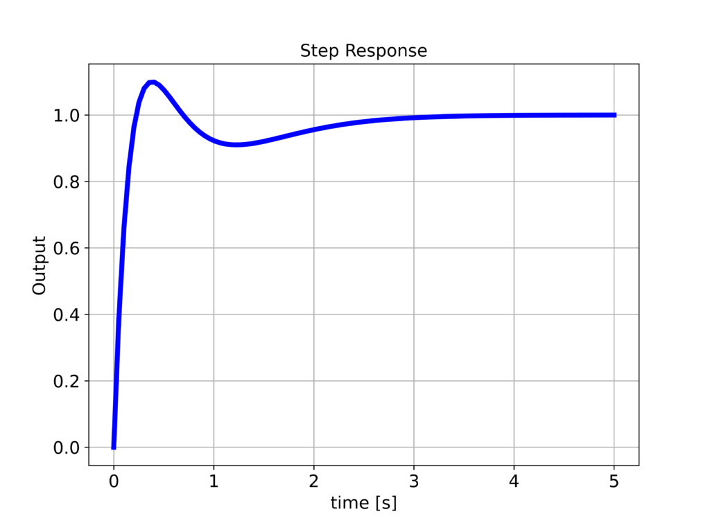
We can observe that we have achieved the desired pole locations. However, we have also introduced zeros in the controller. The real parts of zero are close to the pole $-2$ . Zeros will introduce some oscillations and overshoot in the system response (we will confirm this later on by using simulations). We use the Python Control Systems toolbox to simulate the response of the closed-loop system. The codes are posted at the end of this tutorial. The step response of the closed-loop system is given below.

Figure: Step response of the closed loop system with the closed loop transfer function $W_{cl}$ in (27).

From the figure above, we can observe that there is some overshoot. This overshoot is the direct consequence of the zeros that the controller introduced. Namely, we expected a response that would look similar to the first-order response without an overshoot. This is because the poles are at $s_{1}=-2,\; s_{2}=-3$ and $s_{3}=-4$ , and consequently, we expect a relatively smooth response. However, zeros will introduce the overshoot.

To show that the zeros are the cause of this effect, let us modify the transfer function by removing the zeros and by keeping the DC gain to 1 by adding a constant $24$ in the numerator. The modified transfer function is

(30) $\begin{align*}W_{cl2}=\frac{24}{s^3 + 9 s^2 + 26 s + 24}\end{align*}$

This function does not have zeros and it has a DC gain of $1$ , and consequently, no steady-state error when the step signal is applied. This closed-loop transfer function has the same poles as the transfer function of our closed-loop system. The step response of the modified transfer function $W_{cl2}$ is given below.

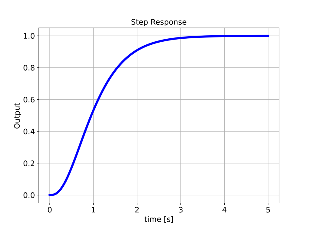in (27).”>Figure: Step response of the modified transfer function $W_{cl2}$ defined in (30) that does not have zeros. Consequently, there is no overshoot.

We can see that the response of the modified system does not suffer from the overshoot. That is, since $W_{cl}$ and $W_{cl2}$ have the same set of poles we can see that the overshoot is mainly due to the zeros of the transfer function $W_{cl}$ .

The Python code used to simulate the closed loop system is given below.


import matplotlib.pyplot as plt
import control as ct
import numpy as np

# this function is used for plotting of responses 
# it generates a plot and saves the plot in a file 

# xAxisVector - time vector
# yAxisVector - response vector
# titleString - title of the plot
# stringXaxis - x axis label 
# stringYaxis - y axis label
# stringFileName - file name for saving the plot, usually png or pdf files

def plottingFunction(xAxisVector,yAxisVector,titleString,stringXaxis,stringYaxis,stringFileName):
    plt.figure(figsize=(8,6))
    plt.plot(xAxisVector,yAxisVector, color='blue',linewidth=4)
    plt.title(titleString, fontsize=14)
    plt.xlabel(stringXaxis, fontsize=14)
    plt.ylabel(stringYaxis,fontsize=14)
    plt.tick_params(axis='both',which='major',labelsize=14)
    plt.grid(visible=True)
    plt.savefig(stringFileName,dpi=600)
    plt.show()
    


# define a transfer function
s = ct.TransferFunction.s
W=1/(s**2+4)
C=(24/s)+22+9*s
# here we define the transfer function

Wcl=W*C/(1+W*C)
Wcl=Wcl.minreal()

print(Wcl)

###############################################################################
# simulate the step response
###############################################################################
timeVector=np.linspace(0,5,100)
timeReturned, systemOutput = ct.step_response(Wcl,timeVector)

# plot the step response
plottingFunction(timeReturned,
                 systemOutput,
                 titleString='Step Response',
                 stringXaxis='time [s]' , 
                 stringYaxis='Output',
                 stringFileName='stepResponse1.png',)
###############################################################################

Wcl.poles()
Wcl.zeros()

# now without zeros

Wcl2= 24*Wcl*1/( 9*s**2 + 22*s + 24)
Wcl2=Wcl2.minreal()
print(Wcl2)


###############################################################################
# simulate the step response
###############################################################################
timeVector=np.linspace(0,5,100)
timeReturned, systemOutput = ct.step_response(Wcl2,timeVector)

# plot the step response
plottingFunction(timeReturned,
                 systemOutput,
                 titleString='Step Response',
                 stringXaxis='time [s]' , 
                 stringYaxis='Output',
                 stringFileName='stepResponse2.png',)
###############################################################################

Problem Statement

Solution

admin

You might also like

Implement Newton’s Method in Python From Scratch by Using SymPy Symbolic Toolbox and Automatic Differentiation

Policy Iteration Algorithm in Python and Tests with Frozen Lake OpenAI Gym Environment- Reinforcement Learning Tutorial

COMSOL Tutorial: Thin-Plate Deformation