 by
by
In this control engineering and control theory tutorial, we explain how the linearization approach can fail when someone is analyzing stability or designing controllers for nonlinear systems. The main motivation for creating this video tutorial comes from the fact that I have noticed that often students, as well as scientists and engineers blindly use the linearization approach when analyzing the stability or designing controllers of nonlinear systems. Consequently, it is very important to explain when we can safely use a linearized model for stability analysis or control system design. The YouTube tutorial accompanying this webpage tutorial is given below.
Lyapunov’s First Method
Consider the nonlinear system
(1) 
where  is the state vector and
  is a nonlinear function that is represented as follows
(2) 
where  ,
,  are scalar functions. Let
  be an equilibrium point around which we linearize the model (1). Let the linearized matrix
  be defined by
(3) 
where the matrix  is the matrix of partial derivatives defined by
(4) 
The linearized system is defined by
(5) 
where  is the relative state-space variable defined with respect to the equilibrium point , that is
(6) 
The following theorem is one of the most important results:
LOCAL STABILITY THEOREM: Consider the nonlinear system (1) and its linearization (5) around the equilibrium point . Then
- If all the eigenvalues of the matrix have strictly negative real parts, then the equilibrium point is asymptotically stable.
- If at least one of the eigenvalues of has a positive real part, then the equilibrium point is unstable.
- If one or more eigenvalues of have zero real parts and no eigenvalues with positive real parts, then we cannot conclude anything about the stability of the equilibrium point by using the linearization approach.
This theorem is very important for the stability analysis by using the linearization approach. Namely, if at least one eigenvalue has a zero real part, and we do not have eigenvalues with positive real parts, then we cannot conclude anything by using the linearization approach. That is, if the linearized model has eigenvalues on the imaginary axis, and no eigenvalue in the right-half of the complex plane, then the linearized model can behave quite differently from the original nonlinear model around the equilibrium point.
Let us illustrate this with the following example
(7) 
The point  and
and  is the equilibrium point of the nonlinear system. To see that, we can see that
  is the solution of the equation
(8) 
Next, we need to linearize the system around this equilibrium point. To do that, we need to recognize that
(9) 
Next, we need to compute the matrix . The matrix is given by
(10) 
Next, we need to determine the eigenvalues of the matrix . The eigenvalues are given by
(11) 
Consequently, the eigenvalues are
(12) 
where  is the imaginary unit. Someone who does not know control system theory will conclude that since the linearized system is stable (marginally stable but not asymptotically stable) nonlinear system will also be stable (marginally stable). Well, this is a wrong conclusion!
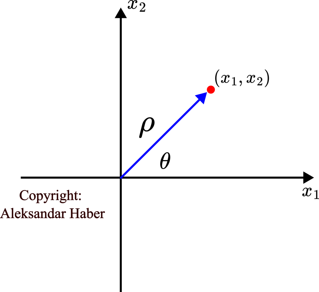
Let us show that. To show that, we need to introduce polar coordinates, since our system will have a much simpler description in the polar coordinates.
(13) 
where  and
and  are the new state-space variables. They are illustrated in the figure below.
Our next task is to express the system dynamics in the polar coordinates (13). To do that, from (13), we have
(14) 
That is,
(15) 
By differentiating the last expression, we obtain
(16) 
Next, let us substitute (15) in the system dynamics (7), as the result, we obtain
(17) 
By substituting (15) and (17) in (16), we obtain
(18) 
That is, the first state equation in the polar coordinates is very simple, and it takes the following form:
(19) 
To derive the second equation for  , we can start from this expression
(20) 
From the last equation, we obtain
(21) 
We know the derivative of  function is given by the following equation
(22) 
By using this expression and by taking the first derivative of (21) with respect to time, we obtain
(23) 
By substituting (7) in the last equation, we obtain
(24) 
The state-space model in the polar coordinates takes a simple form
(25) 
Since  is always positive for positive
  and is by definition always positive, we conclude that the nonlinear system is unstable. However, the linearized model is marginally stable. This example clearly shows the pitfalls of not properly understanding when we can perform stability analysis that is based on linearization.
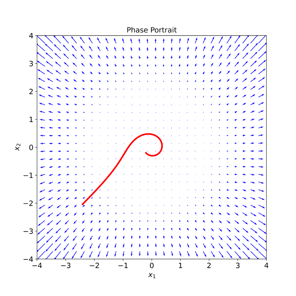
Next, let us plot and compare the phase portraits of linearized and nonlinear models. To plot the phase portraits, we use the Python code posted here. The phase portrait of the nonlinear model (7) is given below.
The phase portrait of the linearized system with the matrix given by the equation (10) is given below.
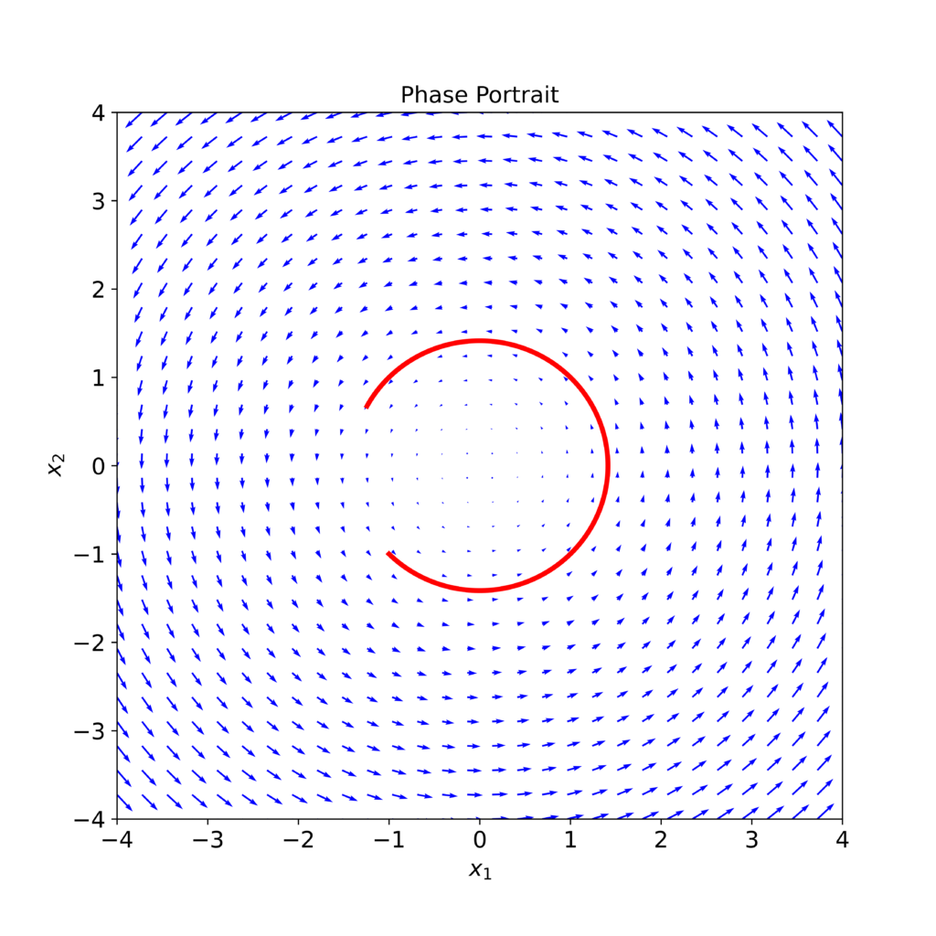 matrix given in (10).